

AI Generated image: Anomaly detection & Recommender Systems
This project explores how Gaussian-based models detect outliers in data and how collaborative filtering powers personalized recommender systems, all within a machine learning framework.
In today's data-driven world, businesses and industries rely on artificial intelligence (AI) to detect unusual patterns and provide personalized recommendations. This project explores two critical machine learning techniques: Anomaly Detection and Recommender Systems.
We implement Gaussian models for anomaly detection, identifying outliers in data such as fraudulent transactions or system failures. Additionally, we build a collaborative filtering-based recommender system, improving personalized suggestions for users in domains like e-commerce, streaming services, and content platforms.
Anomaly detection is the process of identifying rare events or outliers in datasets that do not conform to expected patterns.
We begin by loading the dataset, which contains network performance data (Latency and Throughput). The dataset is stored in a .mat file and is loaded using SciPy.
                    import scipy.io
                    datafile = r'd:\mlprojects\data\ex8data1.mat'
                    mat = scipy.io.loadmat(datafile)
                    X = mat['X']  # Training data
                    ycv = mat['yval']  # Cross-validation labels
                    Xcv = mat['Xval']  # Cross-validation data
Dataset File:
The dataset is stored in ex8data1.mat, a MATLAB/Octave file that contains sample network latency and throughput data. The file is loaded using scipy.io.loadmat(datafile).
Variables Loaded:
X: The training set, a 2D NumPy array where each row represents a network measurement
(Latency & Throughput).ycv: Cross-validation labels, used to evaluate model performance.Xcv: The cross-validation set, used for validation.
Scatter Plot of the Dataset
The following function plots the dataset. Each point represents a network measurement with Latency (X-axis) and Throughput (Y-axis).
                def plotData(myX, newFig=False):
                    if newFig:
                        plt.figure(figsize=(8,6))
                    plt.plot(myX[:,0], myX[:,1], 'b+')
                    plt.xlabel('Latency [ms]', fontsize=16)
                    plt.ylabel('Throughput [mb/s]', fontsize=16)
                    plt.grid(True)
                    plt.show()

                plotData(X)
The output is shown below:
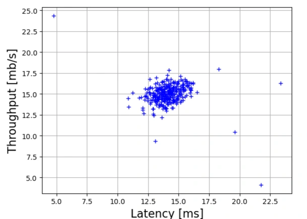
Image 1: Anomaly Detection scatter graph
Explanation:
myX[:,0] represents the Latency (x-axis).myX[:,1] represents the Throughput (y-axis).Computing the Gaussian Probability Density
In this step, we define the function gaus() to compute the probability density for given data points based on Gaussian distribution parameters (mean and variance).
Code Explanation
Python codes:
            def gaus(myX, mymu, mysig2):
                """
                Function to compute the Gaussian probability density for given feature matrix `myX`,
                using mean (`mymu`) and variance (`mysig2`).
                If `mysig2` is a vector, it is converted into a diagonal covariance matrix.
                """
                m = myX.shape[0]  # Number of data points
                n = myX.shape[1]  # Number of features

                # Convert variance to a diagonal covariance matrix if needed
                if np.ndim(mysig2) == 1:
                    mysig2 = np.diag(mysig2)

                # Compute normalization factor
                norm = 1. / (np.power((2 * np.pi), n / 2) * np.sqrt(np.linalg.det(mysig2)))

                # Compute exponent term for Gaussian distribution
                myinv = np.linalg.inv(mysig2)  # Inverse of covariance matrix
                myexp = np.zeros((m, 1))  # Initialize exponent term

                for irow in range(m):  # Iterate over all data points
                    xrow = myX[irow]  # Extract single data point
                    myexp[irow] = np.exp(-0.5 * ((xrow - mymu).T).dot(myinv).dot(xrow - mymu))

                return norm * myexp  # Return computed Gaussian probability
Key Points
Estimating Parameters for Gaussian Distribution
To fit our data into a Gaussian distribution, we estimate the mean (μ) and variance (σ²).
Python codes:
            def getGaussianParams(myX, useMultivariate=True):
                """
                Given a dataset `myX` (m x n), this function computes the mean (μ) and variance (σ²) for each feature.

                It can return:
                - Univariate Gaussian (separate for each feature)
                - Multivariate Gaussian (full covariance matrix)
                """
                m = myX.shape[0]  # Number of examples
                mu = np.mean(myX, axis=0)  # Compute mean for each feature

                if not useMultivariate:  # Univariate Gaussian
                    sigma2 = np.sum(np.square(myX - mu), axis=0) / float(m)  # Variance for each feature
                else:  # Multivariate Gaussian
                    sigma2 = ((myX - mu).T.dot(myX - mu)) / float(m)  # Full covariance matrix

                return mu, sigma2
Key Points
        Python:

        mu, sig2 = getGaussianParams(X, useMultivariate=True)
getGaussianParams() to estimate mean and covariance
matrix of dataset X(mu, sig2) is later used to compute Gaussian probabilitiesTo visualize how the Gaussian distribution fits our dataset, we plot probability contours.
Python codes:
            def plotContours(mymu, mysigma2, newFig=False, useMultivariate=True):
                delta = 0.5  # Grid step size
                myx = np.arange(0, 30, delta)
                yy = np.arange(0, 30, delta)
                meshx, meshy = np.meshgrid(myx, myy)

                # Compute Gaussian probabilities for each point in the grid
                coord_list = [entry.ravel() for entry in (meshx, meshy)]
                points = np.vstack(coord_list).T
                myz = gaus(points, mymu, mysigma2)

                # Reshape probabilities to match grid
                myz = myz.reshape((myx.shape[0], myx.shape[0]))

                if newFig:  # Optionally create a new figure
                    plt.figure(figsize=(6, 4))

                # Define contour levels
                cont_levels = [10**exp for exp in range(-20, 0, 3)]

                # Plot contour lines
                mycont = plt.contour(meshx, meshy, myz, levels=cont_levels)

                plt.title('Gaussian Contours', fontsize=16)
Key Points
Combining Scatter Plot and Contour Plot
Now, we combine scatter and contour plots to visualize our dataset.
Python codes:
            # Create a figure and axis first
            fig, ax = plt.subplots(figsize=(8,6))

            # Scatter plot
            ax.plot(X[:,0], X[:,1], 'b+', label="Data points")
            ax.set_xlabel('Latency [ms]', fontsize=16)
            ax.set_ylabel('Throughput [mb/s]', fontsize=16)

            # Gaussian contours for single-variable Gaussian
            useMV = False
            plotContours(*getGaussianParams(X, useMV), newFig=False, useMultivariate=useMV)

            plt.title('Scatter Plot with Gaussian Contours (Single-variable)')
            plt.legend()
            plt.grid(True)
            plt.show()  # Show first combined plot

            # Create another figure for multivariate Gaussian
            fig, ax = plt.subplots(figsize=(8,6))

            # Scatter plot
            ax.plot(X[:,0], X[:,1], 'b+', label="Data points")
            ax.set_xlabel('Latency [ms]', fontsize=16)
            ax.set_ylabel('Throughput [mb/s]', fontsize=16)

            # Gaussian contours for multivariate Gaussian
            useMV = True
            plotContours(*getGaussianParams(X, useMV), newFig=False, useMultivariate=useMV)

            plt.title('Scatter Plot with Gaussian Contours (Multivariate)')
            plt.legend()
            plt.grid(True)
            plt.show()  # Show second combined plot
After running the above codes, output is a OUTPUT is a Gaussian Contour graph with single variable
Single-variable Gaussian Contour Plot
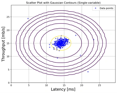
Image 2: Gaussian Contour graph single variable
The first image represents a scatter plot with Gaussian contours generated assuming that the features (Latency and Throughput) are independent. The probability distribution for each feature is computed separately, ignoring any potential correlation between them. As a result, the contours appear as axis-aligned concentric ellipses.
Multivariate Gaussian Contour Plot
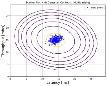
Image 3: Gaussian Contour graph multivariate
The second image represents a scatter plot with Gaussian contours generated using a multivariate Gaussian distribution. Here, the relationship between the features is taken into account, meaning the covariance between Latency and Throughput is considered. This leads to a more realistic representation of the data distribution, potentially causing the contours to tilt or elongate based on the actual covariance.
Single-variable Gaussian:
Multivariate Gaussian:
Conclusion
While the single-variable Gaussian assumption is useful for simpler models, the multivariate Gaussian approach provides a more accurate representation of real-world data distributions, especially when features are correlated.
Compute F1 Score
            def computeF1(predVec, trueVec):
                """
                F1 = 2 * (P*R)/(P+R)
                where P is precision, R is recall
                Precision = "of all predicted y=1, what fraction had true y=1"
                Recall = "of all true y=1, what fraction predicted y=1?
                Note predictionVec and trueLabelVec should be boolean vectors.
                """
                #print predVec.shape
                #print trueVec.shape
                #assert predVec.shape == trueVec.shape

                P, R = 0., 0.
                if float(np.sum(predVec)):
                    P = np.sum([int(trueVec[x]) for x in range(predVec.shape[0]) \
                                if predVec[x]]) / float(np.sum(predVec))
                if float(np.sum(trueVec)):
                    R = np.sum([int(predVec[x]) for x in range(trueVec.shape[0]) \
                                if trueVec[x]]) / float(np.sum(trueVec))

                return 2*P*R/(P+R) if (P+R) else 0
The F1 score balances precision and recall for anomaly detection. It is calculated as:
\[ F1 = 2 \times \frac{P \times R}{P + R} \]
Where:
Select Best Threshold
            def selectThreshold(myycv, mypCVs):
                """
                Function to select the best epsilon value from the CV set
                by looping over possible epsilon values and computing the F1
                score for each.
                """
                # Make a list of possible epsilon values
                nsteps = 1000
                epses = np.linspace(np.min(mypCVs),np.max(mypCVs),nsteps)

                # Compute the F1 score for each epsilon value, and store the best
                # F1 score (and corresponding best epsilon)
                bestF1, bestEps = 0, 0
                trueVec = (myycv == 1).flatten()
                for eps in epses:
                    predVec = mypCVs < eps
                    thisF1 = computeF1(predVec, trueVec)
                    if thisF1 > bestF1:
                        bestF1 = thisF1
                        bestEps = eps

                print("Best F1 is %f, best eps is %0.4g."%(bestF1,bestEps))
                return bestF1, bestEps
This function loops through 1000 possible thresholds (epsilon values) and selects the best one by maximizing the F1 score.
The output of this process is:
Best F1 Score: 0.875
Best Epsilon: 9.075e-05
Compute Probabilities and Threshold
            pCVs = gaus(Xcv, mu, sig2)
            bestF1, bestEps = selectThreshold(ycv,pCVs)

The selected threshold is applied to these probabilities to detect anomalies.
Plot Anomalies
            def plotAnomalies(myX, mybestEps, newFig=False, useMultivariate=True):
                ps = gaus(myX, *getGaussianParams(myX, useMultivariate))
                anoms = np.array([myX[x] for x in range(myX.shape[0]) if ps[x] < mybestEps])

                if newFig:
                    fig, ax = plt.subplots(figsize=(6, 4))
                else:
                    ax = plt.gca()  # Use existing axes

                ax.scatter(anoms[:,0], anoms[:,1], s=80, facecolors='none', edgecolors='r')
The function marks data points as anomalies if their probability is below the selected threshold. These anomalies are displayed as red circles on the graph.
            plt.figure(figsize=(6, 4))  # Create a single figure
            plotData(X, newFig=False)   # Ensure newFig=False
            plotContours(mu, sig2, newFig=False, useMultivariate=True)
            plotAnomalies(X, bestEps, newFig=False, useMultivariate=True)
            plt.show()  # Ensure everything is drawn on the same figure
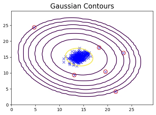
Image 4: Gaussian Contour anamoly detection graph
The final plot combines:
In this analysis, we used a Gaussian-based anomaly detection model to identify unusual data points in a dataset. The process involved:
High-Dimensional Dataset
The dataset used in this anomaly detection example is loaded from an external MATLAB file. The feature set Xpart2 consists of 1000 examples with 11 features each.
Python Codes:
            datafile = r'd:\mlprojects\data\ex8data2.mat'
            mat = scipy.io.loadmat(datafile)
            Xpart2 = mat['X']
            ycvpart2 = mat['yval']
            Xcvpart2 = mat['Xval']
            print('Xpart2 shape is ', Xpart2.shape)
Output:
Xpart2 shape is (1000, 11)
The dataset is loaded using scipy.io.loadmat, and the training data (Xpart2), cross-validation data (Xcvpart2), and labels (ycvpart2) are extracted.
Next, the Gaussian parameters (mean and variance) for anomaly detection are estimated, and probability distributions are computed.
Python Codes:
Python Codes:
            mu, sig2 = getGaussianParams(Xpart2, useMultivariate=False)
            ps = gaus(Xpart2, mu, sig2)
            psCV = gaus(Xcvpart2, mu, sig2)

            # Using Gaussian parameters from the full training set,
            # figure out the p-value for each point in the CV set
            pCVs = gaus(Xcvpart2, mu, sig2)

            # Select the best threshold for anomaly detection
            bestF1, bestEps = selectThreshold(ycvpart2, pCVs)
            anoms = [Xpart2[x] for x in range(Xpart2.shape[0]) if ps[x] < bestEps]
            print('# of anomalies found: ', len(anoms))
Explanation
getGaussianParams(Xpart2, useMultivariate=False): Computes mean and variance for each feature assuming independent Gaussian distribution.gaus(Xpart2, mu, sig2): Computes probability densities for each data point in the training and validation sets.selectThreshold(ycvpart2, pCVs): Determines the best threshold bestEps by optimizing the F1 score.bestEps.
        Best F1 is 0.615385, best eps is 1.379e-18.
        # of anomalies found: 117
The best F1 score of 0.615 is achieved with a threshold of 1.379e-18, resulting in 117 detected anomalies.
Recommender systems enhance user experience by predicting preferences based on past interactions. Recommender systems are widely used in various applications such as movie recommendations, e-commerce, and music streaming. These systems work by analyzing user preferences and suggesting relevant content based on past interactions. They are typically built using collaborative filtering or content-based filtering techniques.
The dataset used in this recommender system consists of movie ratings provided by users:
For example, the average rating for the movie Toy Story is computed as follows:
    print('Average rating for movie 1 (Toy Story): %0.2f' % \
    np.mean([ Y[0][x] for x in range(Y.shape[1]) if R[0][x] ]))
The following code was used to generate the heatmap:
            import matplotlib.pyplot as plt

            fig = plt.figure(figsize=(6,6*(1682./943.)))
            plt.imshow(Y, aspect='auto', cmap='viridis')
            plt.colorbar()
            plt.ylabel('Movies (%d)' % nm, fontsize=20)
            plt.xlabel('Users (%d)' % nu, fontsize=20)
            plt.title('Movie Ratings Heatmap')
            plt.show()
After running the above codes, the heat map is drawn as below:
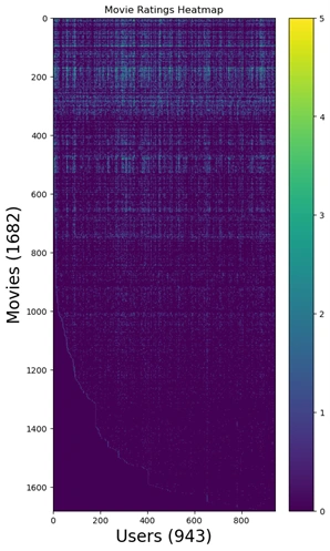
Image 5: Movie recommender rating heat map
To visualize the ratings matrix, a heatmap is generated where:
This visualization helps in understanding rating patterns, spotting popular movies, and detecting sparsity in the dataset.
Collaborative filtering is a machine learning technique used to build recommendation systems by leveraging user-item interactions. It predicts a user's preference for an item based on past behaviors of similar users. This is widely applied in platforms like Netflix and Amazon.
We start by loading the movie rating data and reducing the dataset for faster computation.
            import scipy.io

            datafile = r'd:\mlprojects\data\ex8_movieParams.mat'
            mat = scipy.io.loadmat(datafile)
            X = mat['X']
            Theta = mat['Theta']
            nu = int(mat['num_users'])
            nm = int(mat['num_movies'])
            nf = int(mat['num_features'])

            # Reducing dataset size for faster execution
            nu = 4; nm = 5; nf = 3
            X = X[:nm,:nf]
            Theta = Theta[:nu,:nf]
            Y = Y[:nm,:nu]
            R = R[:nm,:nu]
Explanation: The dataset is loaded, and the matrices for movie features (X) and user preferences (Theta) are extracted. The dataset is then reduced to a smaller size for efficiency.
To use optimization algorithms, we need to flatten and reshape our matrices.
            import numpy as np

            def flattenParams(myX, myTheta):
                return np.concatenate((myX.flatten(), myTheta.flatten()))

            def reshapeParams(flattened_XandTheta, mynm, mynu, mynf):
                reX = flattened_XandTheta[:int(mynm*mynf)].reshape((mynm,mynf))
                reTheta = flattened_XandTheta[int(mynm*mynf):].reshape((mynu,mynf))
                return reX, reTheta
Explanation:
The flattenParams function combines the X and Theta matrices into a single vector for optimization, while reshapeParams reconstructs them back to their original shapes.
            def cofiCostFunc(myparams, myY, myR, mynu, mynm, mynf, mylambda=0.0):
                myX, myTheta = reshapeParams(myparams, mynm, mynu, mynf)
                term1 = np.multiply(myX.dot(myTheta.T), myR)
                cost = 0.5 * np.sum(np.square(term1 - myY))

                # Regularization
                cost += (mylambda / 2.0) * np.sum(np.square(myTheta))
                cost += (mylambda / 2.0) * np.sum(np.square(myX))
                return cost
Explanation:
This function calculates the cost for collaborative filtering by comparing predicted ratings (X * Theta.T) to actual ratings in Y. The cost function also includes regularization terms to prevent overfitting.
            print('Cost with nu = 4, nm = 5, nf = 3 is %0.2f.' %
            cofiCostFunc(flattenParams(X,Theta), Y, R, nu, nm, nf))

            print('Cost with lambda = 1.5 is %0.2f.' %
            cofiCostFunc(flattenParams(X,Theta), Y, R, nu, nm, nf, mylambda=1.5))
Expected Output:
        Cost with nu = 4, nm = 5, nf = 3 is 22.22.
        Cost with lambda = 1.5 is 31.34.
Explanation:
The cost is computed with and without regularization. A higher lambda value increases the cost due to added penalties on complexity.
            def cofiGrad(myparams, myY, myR, mynu, mynm, mynf, mylambda=0.0):
                myX, myTheta = reshapeParams(myparams, mynm, mynu, mynf)
                term1 = np.multiply(myX.dot(myTheta.T), myR) - myY
                Xgrad = term1.dot(myTheta) + mylambda * myX
                Thetagrad = term1.T.dot(myX) + mylambda * myTheta
                return flattenParams(Xgrad, Thetagrad)
Explanation: This function calculates the gradients for X and Theta, which are necessary for optimizing our cost function. Regularization terms are added to prevent overfitting.
Collaborative filtering is a technique used in recommendation systems that predicts user preferences based on past interactions. Instead of relying on explicit attributes of items, it uses matrix factorization to analyze user-item interactions.
The primary idea is to factorize the user-item rating matrix into two lower-dimensional matrices:
The algorithm optimizes these matrices to minimize the difference between predicted and actual ratings using gradient descent. Regularization is applied to prevent overfitting.
Gradient Checking
Verifies computed gradients using numerical approximation.
            def cofiGrad(myparams, myY, myR, mynu, mynm, mynf, mylambda = 0.):
                myX, myTheta = reshapeParams(myparams, mynm, mynu, mynf)
                term1 = myX.dot(myTheta.T)
                term1 = np.multiply(term1,myR)
                term1 -= myY
                Xgrad = term1.dot(myTheta)
                Thetagrad = term1.T.dot(myX)
                Xgrad += mylambda * myX
                Thetagrad += mylambda * myTheta

                return flattenParams(Xgrad, Thetagrad)

            print("Checking gradient with lambda = 0...")
            checkGradient(flattenParams(X,Theta),Y,R,nu,nm,nf)
            print("\nChecking gradient with lambda = 1.5...")
            checkGradient(flattenParams(X,Theta),Y,R,nu,nm,nf,mylambda = 1.5)
Loading Movie Data and User Ratings
            movies = []

            with open('d:\mlprojects\data\movie_ids.txt') as f:       # Movie list
                for line in f:
                    movies.append(' '.join(line.strip('\n').split(' ')[1:]))

            datafile = r'd:\mlprojects\data\ex8_movies.mat'
            mat = scipy.io.loadmat( datafile )
            Y = mat['Y']
            R = mat['R']
            nf = 10   # Use 10 features
Reads movie list from movie_ids.txt and loads the dataset ex8_movies.mat containing:
Y: Movie ratings by usersR: Binary mask (1 if rated, 0 if not)Adding User Ratings
            # Add ratings to the Y matrix, and the relevant row to the R matrix
            myR_row = my_ratings > 0
            Y = np.hstack((Y,my_ratings))
            R = np.hstack((R,myR_row))
            nm, nu = Y.shape
Appends custom ratings to Y and updates the dataset.
Normalizing Ratings
            def normalizeRatings(myY, myR):
                # The mean is only counting movies that were rated
                Ymean = np.sum(myY,axis=1)/np.sum(myR,axis=1)
                Ymean = Ymean.reshape((Ymean.shape[0],1))
                return myY-Ymean, Ymean

            Ynorm, Ymean = normalizeRatings(Y,R)
Ensures that movies with no ratings are properly adjusted by subtracting the mean rating.
Train & extract trained parameters & predict the Model
            # TRAIN
            X = np.random.rand(nm,nf)
            Theta = np.random.rand(nu,nf)
            myflat = flattenParams(X, Theta)

            # Regularization parameter of 10 is used (as used in the homework assignment)
            mylambda = 10.

            # Training the actual model with fmin_cg
            result = scipy.optimize.fmin_cg(cofiCostFunc, x0=myflat, fprime=cofiGrad, \
                                        args=(Y,R,nu,nm,nf,mylambda), \
                                            maxiter=50,disp=True,full_output=True)

            # EXTRACT
            resX, resTheta = reshapeParams(result[0], nm, nu, nf)

            #PREDICT
            prediction_matrix = resX.dot(resTheta.T)
            my_predictions = prediction_matrix[:,-1] + Ymean.flatten()
fmin_cg to optimize X and Theta matrices.X and Theta.T.Sorting and Displaying Top Recommendations
            # Sort my predictions from highest to lowest
            pred_idxs_sorted = np.argsort(my_predictions)
            pred_idxs_sorted[:] = pred_idxs_sorted[::-1]

            print("Top recommendations for you:")
            for i in range(10):
                print('Predicting rating %0.1f for movie %s.' % \
                    (my_predictions[pred_idxs_sorted[i]],movies[pred_idxs_sorted[i]]))

            print("\nOriginal ratings provided:")
            for i in range(len(my_ratings)):
                if my_ratings[i] > 0:
                    print('Rated %d for movie %s.' % (my_ratings[i],movies[i]))
Outputs: Sorts and displays the highest-rated movies for recommendation as shown below:
            Top recommendations:
            Predicting rating 8.3 for movie Shawshank Redemption, The (1994).
            Predicting rating 8.3 for movie Star Wars (1977).
            Predicting rating 8.2 for movie Schindler's List (1993).
            Predicting rating 8.2 for movie Titanic (1997).
            Predicting rating 8.2 for movie Raiders of the Lost Ark (1981).
            Predicting rating 8.2 for movie Wrong Trousers, The (1993).
            Predicting rating 8.1 for movie Close Shave, A (1995).
            Predicting rating 8.1 for movie Usual Suspects, The (1995).
            Predicting rating 8.0 for movie Casablanca (1942).
            Predicting rating 8.0 for movie Good Will Hunting (1997).

            Original ratings provided:
            Rated 4 for movie Toy Story (1995).
            Rated 3 for movie Twelve Monkeys (1995).
            Rated 5 for movie Usual Suspects, The (1995).
            Rated 4 for movie Outbreak (1995).
            Rated 5 for movie Shawshank Redemption, The (1994).
            Rated 3 for movie While You Were Sleeping (1995).
            Rated 5 for movie Forrest Gump (1994).
            Rated 2 for movie Silence of the Lambs, The (1991).
            Rated 4 for movie Alien (1979).
            Rated 5 for movie Die Hard 2 (1990).
            Rated 5 for movie Sphere (1998).
In this project, we explored two powerful machine learning techniques: Anomaly Detection
and Collaborative Filtering for Recommender Systems. Through Anomaly Detection,
we identified rare or suspicious patterns in data using Gaussian distribution-based probability estimations,
making it valuable for fraud detection, network security, and quality control. On the other hand,
Collaborative Filtering allowed us to build personalized recommendation systems by leveraging
user preferences and item similarities, demonstrating its effectiveness in applications like movie
recommendations, e-commerce, and content curation.
These concepts form a strong foundation in machine learning and data science. While our implementation
covered essential techniques, further enhancements can be achieved through deep learning-based
anomaly detection and hybrid recommendation systems. As we move forward,
integrating these advancements can significantly improve accuracy, scalability, and real-world
applicability.
This concludes our study on Anomaly Detection and Recommender Systems. Stay tuned for future projects
exploring more advanced AI and ML concepts! 🚀
1. "Anomaly Detection in Machine Learning" - Research Papers
2. "Recommender Systems: Algorithms and Applications" - AI Journal
I sincerely thank Prof. Andrew NG (DeepLearning.AI, Stanford University) for his inspiring courses that laid the foundation for this project.
 www.HoqueAi.com