

AI Generated image: Bias vs. Variance in Regularized Regression
This project explores how bias and variance influence model performance and how regularization can be used to strike the right balance in polynomial regression models.
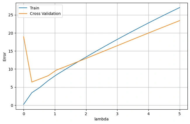
Image 1: High Bias
In this project, we explore the bias-variance trade-off using regularized polynomial regression. The goal is to build a regression model that balances underfitting (high bias) and overfitting (high variance) by adjusting the regularization parameter (λ).
The project follows a structured approach:
By systematically analyzing the impact of λ on model performance, this project provides insights into how to control overfitting and underfitting in machine learning models.
Importing Required Libraries:
            %matplotlib inline
            import numpy as np
            import matplotlib.pyplot as plt
            import scipy.io #Used to load the OCTAVE *.mat files
            import scipy.optimize #fmin_cg to train the linear regression

            import warnings
            warnings.filterwarnings('ignore')
%matplotlib inline command ensures that plots are displayed directly
inside Jupyter Notebook.numpy is imported as np for numerical computations.matplotlib.pyplot is imported as plt for data visualization.scipy.io is used to load MATLAB .mat files, which contain the dataset.scipy.optimize provides optimization functions for training models.warnings.filterwarnings('ignore') suppresses warning messages for a cleaner output.Loading and Preparing the Dataset
            datafile = r'd:\mlprojects\data\ex5data1.mat'
            mat = scipy.io.loadmat(datafile)

            # Training set
            X, y = mat['X'], mat['y']

            # Cross-validation set
            Xval, yval = mat['Xval'], mat['yval']

            # Test set
            Xtest, ytest = mat['Xtest'], mat['ytest']

            # Insert a column of 1's to all of the X's, as usual
            X = np.insert(X, 0, 1, axis=1)
            Xval = np.insert(Xval, 0, 1, axis=1)
            Xtest = np.insert(Xtest, 0, 1, axis=1)
ex5data1.mat, which is in MATLAB format.(X, y)(Xval, yval)(Xtest, ytest)X matrices.Plotting the Training Data
            def plotData():
                plt.figure(figsize=(8,5))
                plt.ylabel('Water flowing out of the dam (y)')
                plt.xlabel('Change in water level (x)')
                plt.plot(X[:,1], y, 'rx')
                plt.grid(True)

            plotData()
OUTPUT: After running codes, the following graph is drawn.
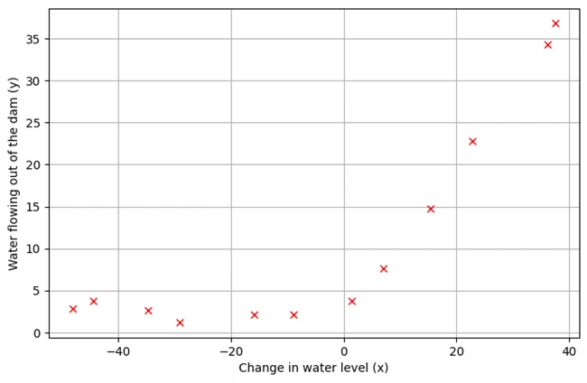
Image 2: Graph 1
1. Description of the Dataset
plotData() is defined to visualize the training data.2. Data Preprocessing
3. Graph Explanation
4. Observations from the Graph
            def h(theta,X): #Linear hypothesis function
                return np.dot(X,theta)

            def computeCost(mytheta,myX,myy,mylambda=0.): #Cost function
                """
                theta_start is an n- dimensional vector of initial theta guess
                X is matrix with n- columns and m- rows
                y is a matrix with m- rows and 1 column
                """
                m = myX.shape[0]
                myh = h(mytheta,myX).reshape((m,1))
                mycost = float((1./(2*m)) * np.dot((myh-myy).T,(myh-myy)))
                regterm = (float(mylambda)/(2*m)) * float(mytheta[1:].T.dot(mytheta[1:]))
                return mycost + regterm
Expllanation:
h(theta, X): Implements the linear hypothesis
function \(
h_{\theta}(x) = \theta^T X
\).
computeCost(mytheta, myX, myy, mylambda=0.):
(Note: Regularization does not apply to \( \theta_0 \), the bias term.)
Computing Cost with Given \( \theta_0 \) Values
Using codes:
            #Using theta initialized at [1; 1], and lambda = 1.
            mytheta = np.array([[1.],[1.]])
            print(computeCost(mytheta,X,y,mylambda=1.))

            OUTPUT:
            303.9931922202643
Explanation:
303.9931922202643This value represents the error of the model before training.
            def computeGradient(mytheta,myX,myy,mylambda=0.):
                mytheta = mytheta.reshape((mytheta.shape[0],1))
                m = myX.shape[0]
                #grad has same shape as myTheta (2x1)
                myh = h(mytheta,myX).reshape((m,1))
                grad = (1./float(m))*myX.T.dot(h(mytheta,myX)-myy)
                regterm = (float(mylambda)/m)*mytheta
                regterm[0] = 0 #don't regulate bias term
                regterm.reshape((grad.shape[0],1))
                return grad + regterm

                #Here's a wrapper for computeGradient that flattens the output
                #This is for the minimization routine that wants everything flattened

            def computeGradientFlattened(mytheta,myX,myy,mylambda=0.):
                return computeGradient(mytheta,myX,myy,mylambda=0.).flatten()
Explanation:
1. Function computeGradient(mytheta, myX, myy, mylambda=0.):
2. Function computeGradientFlattened():
scipy.optimize.Computing the Gradient for \( \theta \) = [1,1]
            # Using theta initialized at [1; 1] we would expect to see a
            # gradient of [-15.303016; 598.250744] (with lambda=1)
            mytheta = np.array([[1.],[1.]])
            print(computeGradient(mytheta,X,y,1.))
OUTPUT:
\( \left[
\begin{array}{c}
-15.303016 \\
598.250744
\end{array}
\right] \)
Note: This tells us how \( \theta_0 \) should be updated to minimize the cost.
Fitting linear regression:
Codes used:
            def optimizeTheta(myTheta_initial, myX, myy, mylambda=0.,print_output=True):
                fit_theta = scipy.optimize.fmin_cg(computeCost,x0=myTheta_initial,\
                                                    fprime=computeGradientFlattened,\
                                                    args=(myX,myy,mylambda),\
                                                    disp=print_output,\
                                                    epsilon=1.49e-12,\
                                                    maxiter=1000)
                fit_theta = fit_theta.reshape((myTheta_initial.shape[0],1))
                return fit_theta
Function optimizeTheta():
(fmin_cg) to find
the best \( \theta_0 \) values that minimize the cost function.Running Optimization
            mytheta = np.array([[1.],[1.]])
            fit_theta = optimizeTheta(mytheta,X,y,0.)

            OUTPUT:
            Optimization terminated successfully.
                    Current function value: 22.373906
                    Iterations: 18
                    Function evaluations: 28
                    Gradient evaluations: 28
Explanation:
Plotting the Fitted Line
            plotData()
            plt.plot(X[:,1],h(fit_theta,X).flatten())
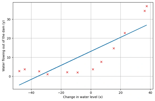
Image 3: Graph 2
Graph Descriptions:
plotData() to re-plot the data points.Key Takeaways:
Generating the Learning Curve:
Python codes:
            def plotLearningCurve():
                """
                Loop over first training point, then first 2 training points, then first 3 ...
                and use each training-set-subset to find trained parameters.
                With those parameters, compute the cost on that subset (Jtrain)
                remembering that for Jtrain, lambda = 0 (even if you are using regularization).
                Then, use the trained parameters to compute Jval on the entire validation set
                again forcing lambda = 0 even if using regularization.
                Store the computed errors, error_train and error_val and plot them.
                """
                initial_theta = np.array([[1.],[1.]])
                mym, error_train, error_val = [], [], []
                for x in range(1,13,1):
                    train_subset = X[:x,:]
                    y_subset = y[:x]
                    mym.append(y_subset.shape[0])
                    fit_theta = optimizeTheta(initial_theta,train_subset,y_subset,mylambda=0.,print_output=False)
                    error_train.append(computeCost(fit_theta,train_subset,y_subset,mylambda=0.))
                    error_val.append(computeCost(fit_theta,Xval,yval,mylambda=0.))

                plt.figure(figsize=(8,5))
                plt.plot(mym,error_train,label='Train')
                plt.plot(mym,error_val,label='Cross Validation')
                plt.legend()
                plt.title('Learning curve for linear regression')
                plt.xlabel('Number of training examples')
                plt.ylabel('Error')
                plt.grid(True)
The function plotLearningCurve() is designed to visualize the
bias-variance tradeoff by plotting the learning curve. Here's
what it does:
optimizeTheta().(Jtrain):
computeCost() on the entire
validation set with lambda = 0.(Jval):
computeCost() on the entire
validation set with lambda = 0.(error_train and error_val)
for plotting.Running the Learning Curve Function
            plotLearningCurve()

            OUTPUT:
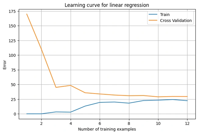
Image 4: Graph 3
Graph Descriptions:
plotLearningCurve() to generate and display
the learning curve.Polynomial regression allows us to capture complex, non-linear relationships
that simple linear regression cannot.
In this section, we apply polynomial regression (degree = 5) and observe
how it fits the data.
Polynomial Features and Feature Scaling:
Optimization Process:
Polynomial regression:
Python codes:
                def genPolyFeatures(myX,p):
                """
                    Function takes in the X matrix (with bias term already included as the first column)
                    and returns an X matrix with "p" additional columns.
                    The first additional column will be the 2nd column (first non-bias column) squared,
                    the next additional column will be the 2nd column cubed, etc.
                    """
                    newX = myX.copy()
                    for i in range(p):
                        dim = i+2
                        newX = np.insert(newX,newX.shape[1],np.power(newX[:,1],dim),axis=1)
                    return newX

                def featureNormalize(myX):
                    """
                    Takes as input the X array (with bias "1" first column), does
                    feature normalizing on the columns (subtract mean, divide by standard deviation).
                    Returns the feature-normalized X, and feature means and stds in a list
                    Note this is different than my implementation in assignment 1...
                    I didn't realize you should subtract the means, THEN compute std of the
                    mean-subtracted columns.
                    Doesn't make a huge difference, I've found
                    """

                    Xnorm = myX.copy()
                    stored_feature_means = np.mean(Xnorm,axis=0) #column-by-column
                    Xnorm[:,1:] = Xnorm[:,1:] - stored_feature_means[1:]
                    stored_feature_stds = np.std(Xnorm,axis=0,ddof=1)
                    Xnorm[:,1:] = Xnorm[:,1:] / stored_feature_stds[1:]
                    return Xnorm, stored_feature_means, stored_feature_stds
Function 1: genPolyFeatures(myX, p)
X and generates polynomial
features up to degree p.x^p.Function 2: featureNormalize(myX)
Python codes:
                #Generate an X matrix with terms up through x^8
                #(7 additional columns to the X matrix)

                global_d = 5
                newX = genPolyFeatures(X,global_d)
                newX_norm, stored_means, stored_stds = featureNormalize(newX)
                #Find fit parameters starting with 1's as the initial guess
                mytheta = np.ones((newX_norm.shape[1],1))
                fit_theta = optimizeTheta(mytheta,newX_norm,y,0.)

                OUTPUT:
                Optimization terminated successfully.
                        Current function value: 0.198053
                        Iterations: 76
                        Function evaluations: 152
                        Gradient evaluations: 152
Code Explanation:
global_d = 5 → Uses polynomials up to degree 5 (x² to x⁶).genPolyFeatures(X, global_d) → Generates new X with
polynomial terms.featureNormalize(newX) → Normalizes the dataset.optimizeTheta() to minimize cost and find the
best theta values.
        Optimization terminated successfully.
        Current function value: 0.198053
        Iterations: 76
        Function evaluations: 152
        Gradient evaluations: 152
Interpretation:
The cost function reached 0.198 after 76 iterations, meaning the polynomial regression model is learning well.
Python codes:
            def plotFit(fit_theta,means,stds):
                """
                Function that takes in some learned fit values (on feature-normalized data)
                It sets x-points as a linspace, constructs an appropriate X matrix,
                un-does previous feature normalization, computes the hypothesis values,
                and plots on top of data
                """
                n_points_to_plot = 50
                xvals = np.linspace(-55,55,n_points_to_plot)
                xmat = np.ones((n_points_to_plot,1))

                xmat = np.insert(xmat,xmat.shape[1],xvals.T,axis=1)
                xmat = genPolyFeatures(xmat,len(fit_theta)-2)
                #This is undoing feature normalization
                xmat[:,1:] = xmat[:,1:] - means[1:]
                xmat[:,1:] = xmat[:,1:] / stds[1:]
                plotData()
                plt.plot(xvals,h(fit_theta,xmat),'b--')

                plotFit(fit_theta,stored_means,stored_stds)
Oouput Graph:
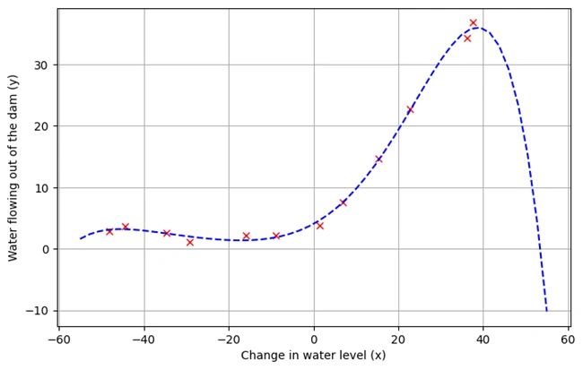
Image 5: Graph 4
Graph Descriptions:
Function: plotFit(fit_theta, means, stds)
xvals from -55 to 55).genPolyFeatures().undoes scaling).h().✅ Final Output: A Graph Showing the Polynomial Regression Fit
This function plotPolyLearningCurve is used to plot the learning curve for Polynomial Regression. The learning curve helps analyze the bias-variance tradeoff by comparing training error and cross-validation error as the number of training examples increases.
Python codes:
                def plotPolyLearningCurve(mylambda=0.):

                    initial_theta = np.ones((global_d+2,1))
                    mym, error_train, error_val = [], [], []
                    myXval, dummy1, dummy2 = featureNormalize(genPolyFeatures(Xval,global_d))

                    for x in range(1,13,1):
                        train_subset = X[:x,:]
                        y_subset = y[:x]
                        mym.append(y_subset.shape[0])
                        train_subset = genPolyFeatures(train_subset,global_d)
                        train_subset, dummy1, dummy2 = featureNormalize(train_subset)
                        fit_theta = optimizeTheta(initial_theta,train_subset,y_subset,mylambda=mylambda,print_output=False)
                        error_train.append(computeCost(fit_theta,train_subset,y_subset,mylambda=mylambda))
                        error_val.append(computeCost(fit_theta,myXval,yval,mylambda=mylambda))

                    plt.figure(figsize=(8,5))
                    plt.plot(mym,error_train,label='Train')
                    plt.plot(mym,error_val,label='Cross Validation')
                    plt.legend()
                    plt.title('Polynomial Regression Learning Curve (lambda = 0)')
                    plt.xlabel('Number of training examples')
                    plt.ylabel('Error')
                    plt.ylim([0,100])
                    plt.grid(True)

                    plotPolyLearningCurve()
1. Initialize Variables:
      Python:

      initial_theta = np.ones((global_d+2,1))
      mym, error_train, error_val = [], [], []
initial_theta: A vector initialized with ones, used as the initial guess for optimization.mym: Stores the number of training examples.error_train & error_val: Lists to store training and validation errors.2. Prepare the Validation Set (Xval):
            Python:

            myXval, dummy1, dummy2 = featureNormalize(genPolyFeatures(Xval,global_d))
Xval into polynomial features up to degree global_d.3. Loop Over Different Training Set Sizes:
            Python:

            for x in range(1,13,1):
4. Generate Polynomial Features & Normalize:
            Python:

            train_subset = X[:x,:]
            y_subset = y[:x]
            train_subset = genPolyFeatures(train_subset,global_d)
            train_subset, dummy1, dummy2 = featureNormalize(train_subset)
(X[:x,:] and y[:x]).5. Optimize the Model (Train Parameters):
            Python:

            fit_theta = optimizeTheta(initial_theta,train_subset,y_subset,mylambda=mylambda,print_output=False)
fit_theta.6. Compute Training and Validation Errors:
            Python:

            error_train.append(computeCost(fit_theta,train_subset,y_subset,mylambda=mylambda))
            error_val.append(computeCost(fit_theta,myXval,yval,mylambda=mylambda))
error_train: Computes cost on the subset of training data.error_val: Computes cost on the full validation set.7. Plot the Learning Curve:
            Python:

            plt.figure(figsize=(8,5))
            plt.plot(mym,error_train,label='Train')
            plt.plot(mym,error_val,label='Cross Validation')
            plt.legend()
            plt.title('Polynomial Regression Learning Curve (lambda = 0)')
            plt.xlabel('Number of training examples')
            plt.ylabel('Error')
            plt.ylim([0,100])
            plt.grid(True)
Output:
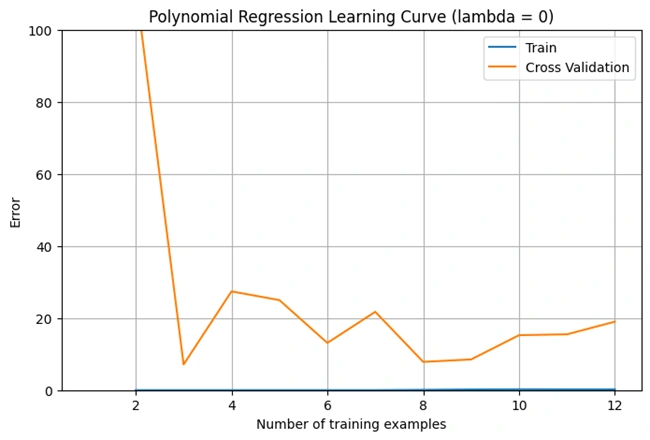
Image 6: Graph 4
Explanation of the Learning Curve (Lambda = 0)
This graph represents the learning curve for polynomial regression when λ (lambda) = 0 (no regularization). It shows how the cross-validation error changes as the number of training examples increases.
1. High Initial Error:
2. Error Drops Quickly:
3. Fluctuations in Error:
4. Indication of Overfitting:
Conclusion:
This section adjusts the regularization parameter (lambda = 1) and evaluates its effect on polynomial regression. The process includes:
Python codes:
                #Try Lambda = 1
                mytheta = np.zeros((newX_norm.shape[1],1))
                fit_theta = optimizeTheta(mytheta,newX_norm,y,1)
                plotFit(fit_theta,stored_means,stored_stds)
                plotPolyLearningCurve(1.)

                OUTPUT:
                Current function value: 8.042488
                        Iterations: 5
                        Function evaluations: 71
                        Gradient evaluations: 60

                Loading the two graphs:
Explanation of the Codes
1. Initializing Theta:
                Python:

                mytheta = np.zeros((newX_norm.shape[1],1))
mytheta is created.2. Optimizing Theta for Lambda = 1:
                Python:

                fit_theta = optimizeTheta(mytheta, newX_norm, y, 1)
3. Plotting the Polynomial Fit:
                Python:

                plotFit(fit_theta, stored_means, stored_stds)
Output:Polynomial Regression Fit Curve with λ = 1
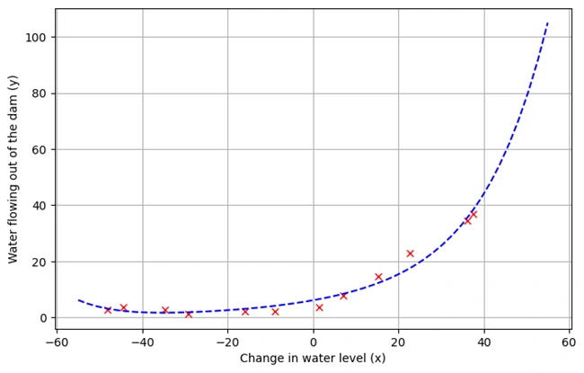
Image 7: Polynomial Regression Fit Curve with λ = 1
Explanation of the Polynomial Regression Fit Curve with λ = 1
Polynomial regression model fitted to the dataset with regularization (λ = 1). The red markers represent actual data points, while the blue dashed curve represents the model’s prediction. Regularization helps control overfitting, ensuring a smoother and more generalized fit.
4. Plotting the Learning Curve for λ = 1:
                Python:

                plotPolyLearningCurve(1.)
Output: Polynomial Regression Learning Curve, λ = 1
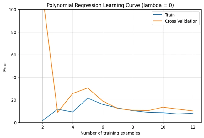
Image 8: Polynomial Regression Learning Curve, λ = 1
Explanation of the Polynomial Regression Learning Curve, λ = 1
Learning curve analysis for polynomial regression with regularization (λ = 1). The training error (blue) and cross-validation error (orange) converge as the number of training examples increases, demonstrating improved generalization and reduced variance.
Python codes:
                #Try Lambda = 100
                #Note after one iteration, the lambda of 100 penalizes the theta params so hard
                #that the minimizer loses precision and gives up...
                #so the plot below is NOT indicative of a successful fit
                mytheta = np.random.rand(newX_norm.shape[1],1)
                fit_theta = optimizeTheta(mytheta,newX_norm,y,100.)
                plotFit(fit_theta,stored_means,stored_stds)

                OUTPUT:
                Current function value: 131.414491
                    Iterations: 0
                    Function evaluations: 38
                    Gradient evaluations: 27
Explanation of the Codes
In this cell, you are testing the impact of a high regularization parameter λ = 100 on polynomial regression.
                Python:

                mytheta = np.random.rand(newX_norm.shape[1],1)
θ with random values. This is different from
earlier codes, where θ was initialized to zeros.
                Python:

                fit_theta = optimizeTheta(mytheta, newX_norm, y, 100.)
(Iterations: 0), meaning it failed
to improve the model.
                Python:

                plotFit(fit_theta, stored_means, stored_stds)
Output: Polynomial Regression Learning Curve, λ = 1
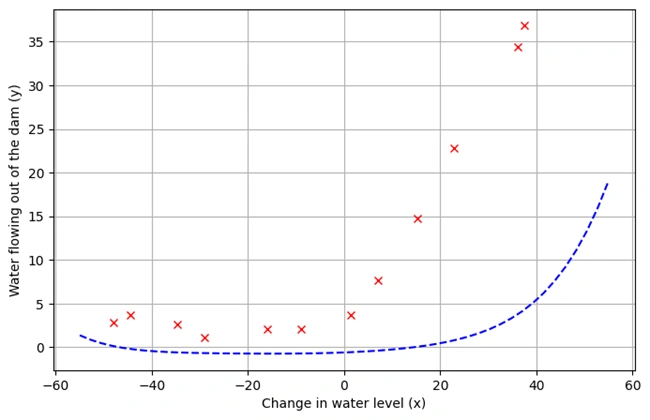
Image 9: Polynomial regression model with high regularization (λ = 100)
Explanation of the graph
Graph showing what impact of High Regularization on Polynomial Regression:
Polynomial regression model with high regularization (λ = 100). The model fails to capture the data trend due to excessive penalization of parameters, resulting in severe underfitting. The optimization process does not complete successfully, demonstrating the negative impact of overly strong regularization.
This is a classic example of over-regularization, where the model becomes too simple and fails to capture important patterns in the data.
Training and Validation Error Calculation:
Python codes:
                #lambdas = [0., 0.001, 0.003, 0.01, 0.03, 0.1, 0.3, 1., 3., 10.]
                lambdas = np.linspace(0,5,20)
                errors_train, errors_val = [], []
                for mylambda in lambdas:
                    newXtrain = genPolyFeatures(X,global_d)
                    newXtrain_norm, dummy1, dummy2 = featureNormalize(newXtrain)
                    newXval = genPolyFeatures(Xval,global_d)
                    newXval_norm, dummy1, dummy2 = featureNormalize(newXval)
                    init_theta = np.ones((newX_norm.shape[1],1))
                    fit_theta = optimizeTheta(mytheta,newXtrain_norm,y,mylambda,False)
                    errors_train.append(computeCost(fit_theta,newXtrain_norm,y,mylambda=mylambda))
                    errors_val.append(computeCost(fit_theta,newXval_norm,yval,mylambda=mylambda))
Explanation of the codes:
The codes run polynomial regression for different values of the regularization parameter λ (lambda) and records the corresponding training and cross-validation errors.
lambdas = np.linspace(0,5,20) → Generates 20 evenly spaced values
of λ between 0 and 5.Plotting the Errors vs. Lambda
                Python:

                plt.figure(figsize=(8,5))
                plt.plot(lambdas,errors_train,label='Train')
                plt.plot(lambdas,errors_val,label='Cross Validation')
                plt.legend()
                plt.xlabel('lambda')
                plt.ylabel('Error')
                plt.grid(True)
This code plots the errors from the previous step to visualize the impact of different λ values on model performance.
Output: Optimal Regularization Parameter (λ) Using Cross-Validatio
Image 9: Effect of regularization (λ) on polynomial regression performance.
This graph illustrates the effect of different regularization strengths (λ) on training and validation errors.
The blue line represents training error, while the orange line represents cross-validation error. The optimal λ value is where validation error is minimized, balancing bias and variance.
The graph typically follows this trend:
This project highlights the importance of regularization in polynomial regression. Key takeaways include:
Through this exercise, we demonstrated how cross-validation helps in selecting the right λ, making the model more generalizable to unseen data. This method is essential for improving model robustness in real-world machine learning applications.
I sincerely thank Prof. Andrew NG (DeepLearning.AI, Stanford University) for his inspiring courses that laid the foundation for this project.
 www.HoqueAi.com