
Self-driving car deep learning project using INVIDIA's Convolutional Neural Network Concepts.
Simulator: Udacity Self-Driving Car Simulator
📹 Video created by HoqueAI during exercise in Udacity Self-Driving Car Simulator.
🎵 Background music: Copyright-free music, Emotional-piano-music-256262.mp3, from Pixabay.com
This project demonstrates the implementation of a self-driving car system using deep learning and real-time image processing. The model is integrated into a virtual simulation environment for live testing.
Autonomous vehicles are one of the most groundbreaking innovations of the 21st century. With AI-powered systems at their core, self-driving cars are revolutionizing transportation, promising safer and more efficient roadways.
Self-driving cars rely on a combination of Artificial Intelligence (AI), sensors, cameras, radar, and LiDAR to interpret their surroundings and navigate safely.
a) We shall download dataset from from Github site of Audacity.
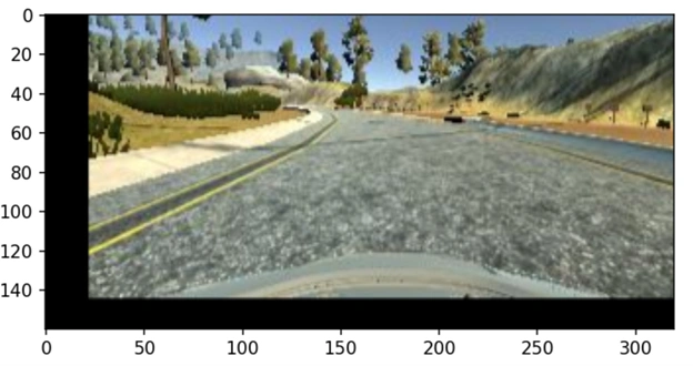
b) Model Train in this video: Train the model on training track and run on as shown below:
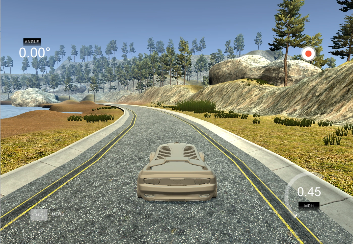
Autonomous driving with convolutional neural networks. Training track: comparatively easy track
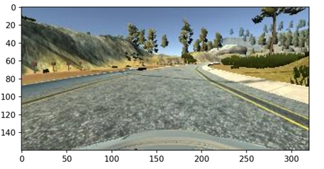
c) In another next video We shall train the model on a rough hilly difficult track and run
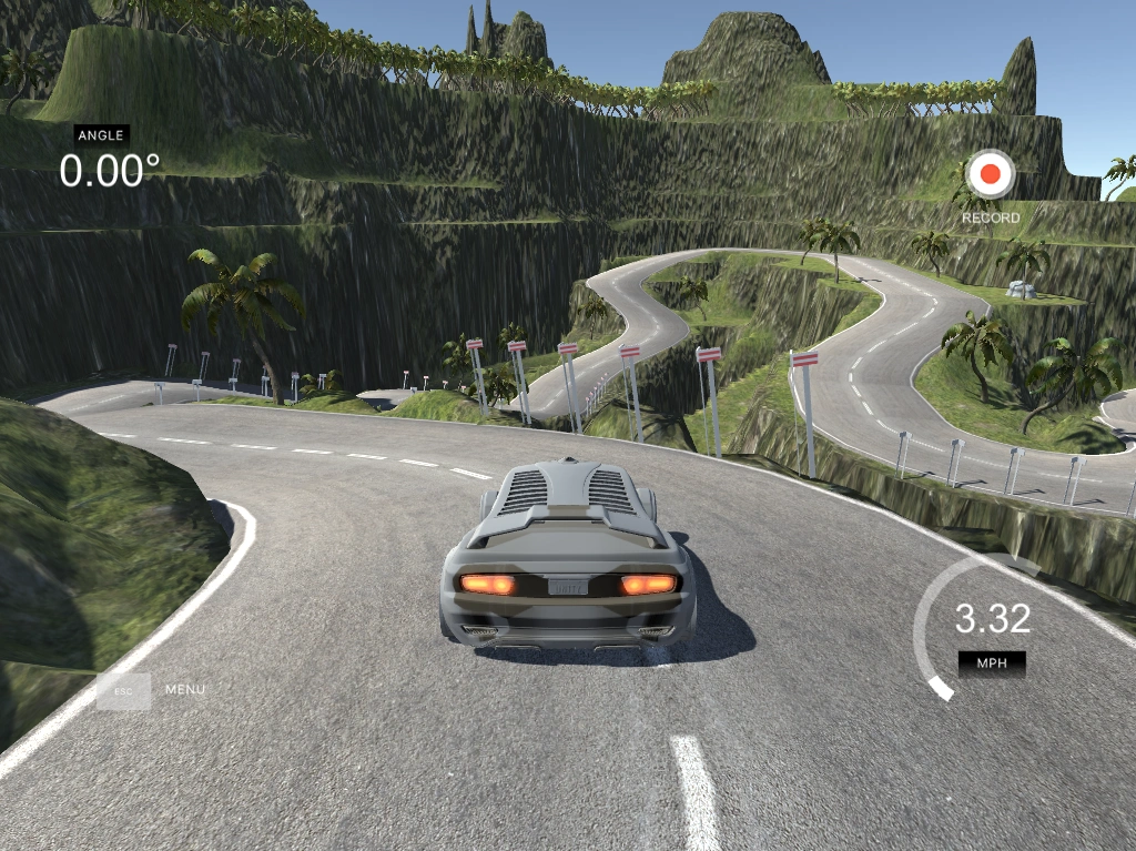
Autonomous driving with convolutional neural networks. Tough hilly difficult track: Not so easy.
We learn to drive not just by reading rules, but by observing, experiencing, and practicing
on the road. For years, we watch how others handle steering, follow traffic lights, respond
to signs, slow down near crosswalks, and accelerate on open roads.
During our driving lessons, we actively absorb critical cues—like recognizing pedestrian
zones, interpreting lane markings, understanding different types of center lines, and knowing exactly
when to stop or go. Our brains continuously collect, process, and store this information,
building a mental model of real-world driving.
Once we pass our driving test, we’re ready to drive with confidence—relying on this rich dataset encoded
in our memory.
In a similar way, we train self-driving models. Instead of human brains, we use powerful neural networks.
These models learn from road data, including images, sensor readings, and driving
patterns—mimicking the way we learn. With enough training, they too can make intelligent driving
decisions, navigate traffic, and adapt to dynamic road conditions.
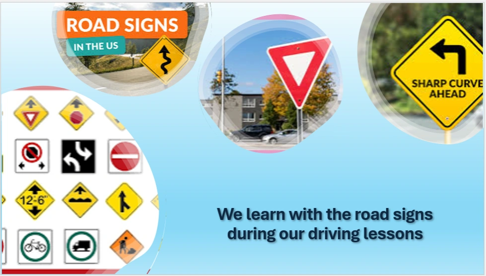
Image showing different road signs
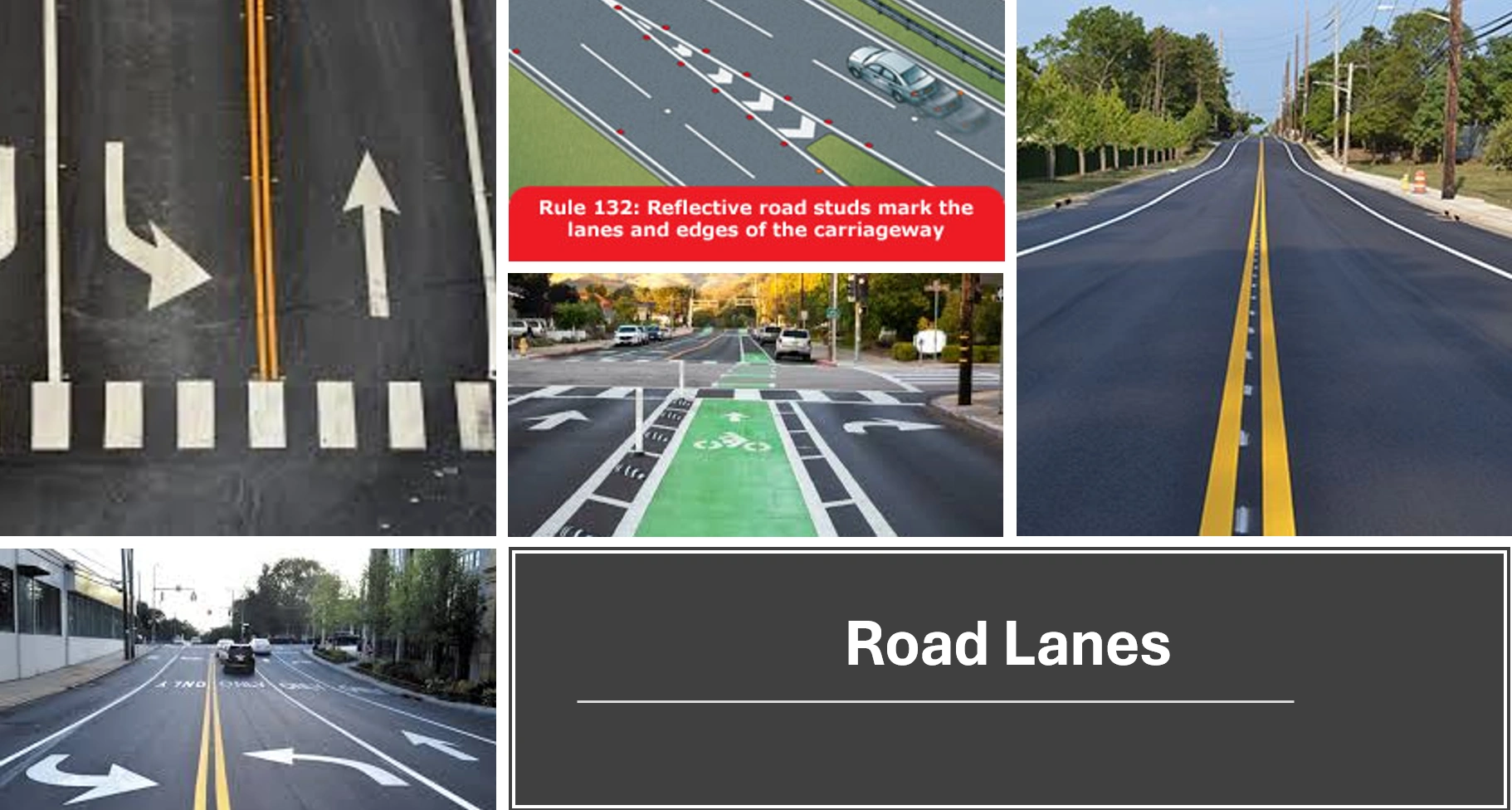
Image showing different road marks and lanes. Road lane detection using deep learning
NVIDIA’s approach involves feeding steering angle data along with images from three cameras—left, center, and right—into a Convolutional Neural Network (CNN). The model is then trained using these inputs and optimized parameters to learn and generalize driving behavior effectively.
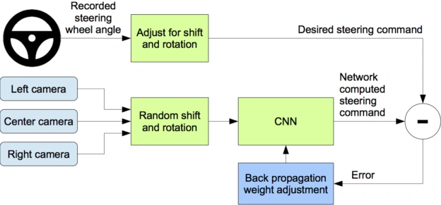
Flow diagram NVIDIA's Approach.
The first and essential step in building a self-driving car model is collecting the dataset. To do this, we use the Udacity Self-Driving Car Simulator, which helps simulate road environments and collect real-time driving data.
You can download the simulator from the official GitHub repository:
🔗 Udacity Self-Driving Car Simulator (GitHub)
It is available for all platforms, including:
👉 For this demo, we will use the Windows version.
After downloading the simulator, click on beta-simulator icon and select Screen resolution and Graphics quality. Click on the play button as shown below:
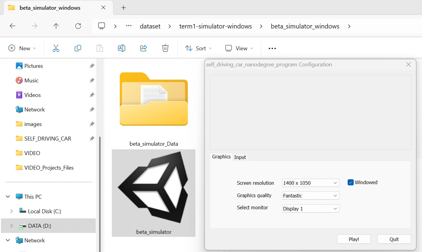
Configure simulator.
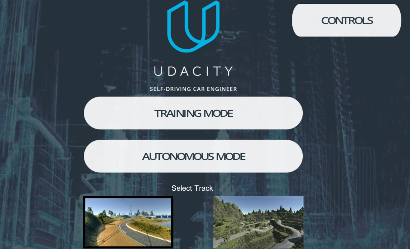
Simulator menu
There are two modes:
There are two tracks:
Select: Left easy track.
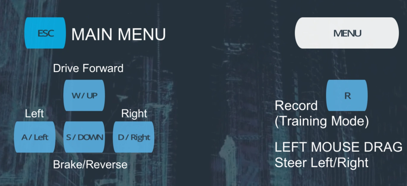
Click: Training mode.
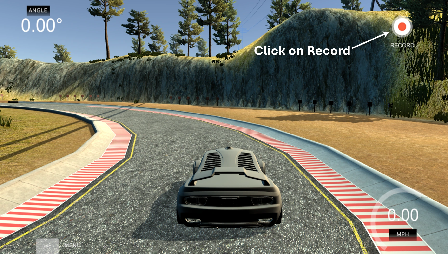
Click on Record button
Select: Select a folder to save recorded taining data.
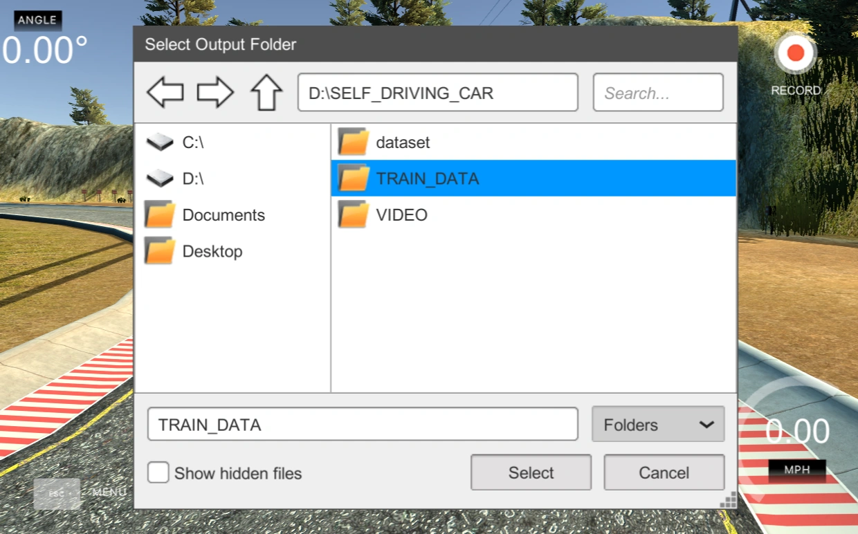
Select TRAIN_DATA Folder
Select Train Navigation
Navigations:
VIDEO during data collection cycles using Udacity Self-Driving Car Simulator.
📹 Video created by HoqueAI during exercise in Udacity Self-Driving Car Simulator.
🎵 Background music: Copyright-free music, Pagol Mon Bangla Music Sound, from Pixabay.com
To run the video, please click on the play button
NOTE:In this way run the training cycles 3 to 5 times
During simulation, we have manually controlled the car and collect sensor data including:
After driving a few laps on the test track, a folder was created with:
driving_log.csv – Contains metadata (image path, steering, throttle, brake, speed)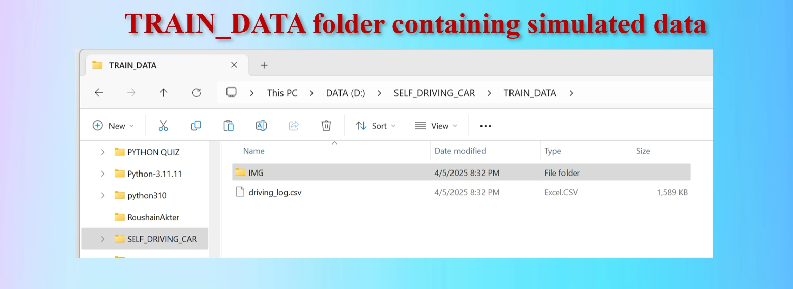
Select TRAIN_DATA Folder
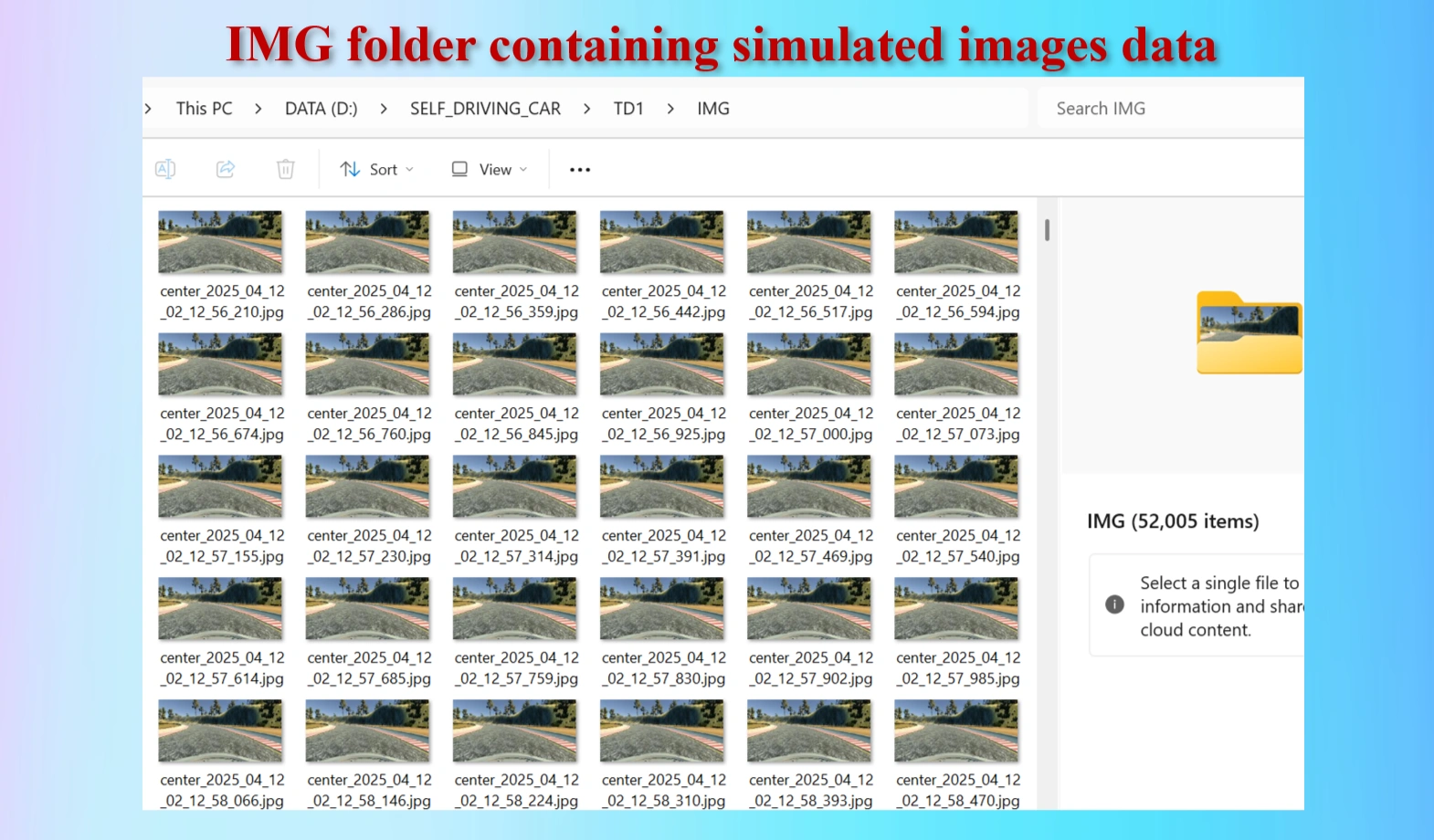
The IMG contains 52,005 images
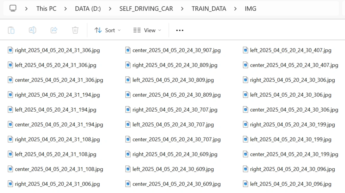
IMG containing 52,005 images
Out of 52,005 images, some of the images are from Central camera, some of them from Left camera and some of them from Right camara.
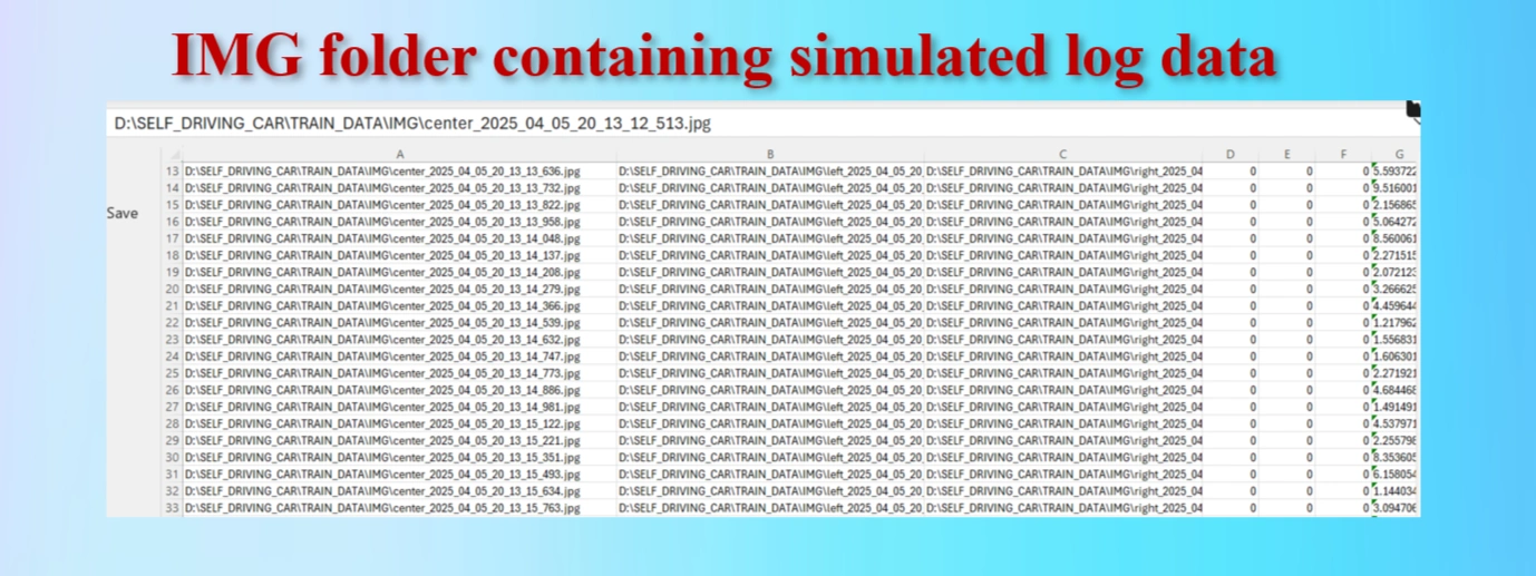
Model training log files in CSV format
Welcome back, road coders! In this exciting third part of our self-driving car simulation series using Convolutional Neural Networks, we're diving into a must-do step—visualizing and balancing our data to prevent steering bias and boost model performance. Let’s gear up! 💡
Before hitting the road, we need to see how our steering data is distributed. If our dataset has too many left turns and not enough right ones, our car might end up favoring the left lane forever! That’s a no-go. To fix this, we split our continuous steering values (ranging from -1 to 1) into bins—like buckets—so we can spot imbalance visually using a bar graph.
We’ll build a balance_data() function in our utilities.py. It’ll
plot the distribution of steering angles, with a toggle option (display=True)
so we can turn graphs on or off when needed.
We define 31 bins—why odd? Because we want zero (driving straight) to sit
right in the middle. Using numpy.histogram(), we break down how many data
points fall into each bin, giving us a clearer picture of what our dataset looks like behind
the scenes.
When we run this, we notice something weird—zero isn’t represented in our bin edges. But going straight is the most common driving behavior, so this is a big red flag. Our current setup misses a crucial piece of the data puzzle.
To fix this, we’ll craft a custom binning method that ensures zero is clearly captured, and all steering angles are evenly balanced. This will train our model to handle curves and straightaways like a pro.
Ready to fine-tune your AI driver? Let’s hit the road to Part 4! 🛣️🚘
To steer our self-driving model in the right direction—literally—we must fix an issue that could throw it off course: steering bias. Our dataset had a massive spike at zero steering angle, meaning the car was mostly driving straight. While that’s realistic on highways, it can hurt performance during curves and turns.
To understand this imbalance, we plotted a histogram using 31 bins, centered
around zero. But we didn’t stop there! We created precise center values
using:
center = (bins[1:] + bins[:-1]) / 2This gave us a beautifully balanced spread, with 0 at the center, extending to ±0.96—representing left and right steering extremes.
Before applying any data balancing techniques, we analyzed the distribution of steering angle values captured in the dataset. The values were grouped into 31 bins to better understand how frequently the vehicle was turning left, right, or driving straight.
The midpoints of these bins are visualized below. Notice the center point marked as "0."—this represents straight driving, which dominates most real-world driving data. The even spread of values across the negative and positive angles reflects a healthy range of left and right turns as well.
This visualization laid the foundation for our data pruning strategy. By identifying and removing overrepresented angles (especially around 0°), we significantly reduced redundancy and enhanced our model’s ability to learn from turns and edge cases.
Python
        def balanceData(data, display=True): ## FOR ALL MUST
            nBins = 31
            samplesPerBin = 3000
            hist, bins = np.histogram(data['Steering'], nBins)
            if display:
                center = (bins[:-1] + bins[1:]) * 0.5
                print(center)

                plt.figure(figsize=(10, 4))
                plt.bar(center, hist, width = 0.06, color='salmon')
                plt.plot((-1,1), (samplesPerBin, samplesPerBin))
                plt.title('Steering Angle Distribution After Pruning')
                plt.xlabel('Steering Angle')
                plt.ylabel('Number of Images')
                plt.show()
In real-world driving data, steering angles tend to cluster heavily around zero—indicating
that most driving is done in a straight line. While this reflects actual road behavior,
using such skewed data without filtering can cause our self-driving model to become biased
and predict straight paths excessively, even when turns are necessary.
To counter this imbalance, we implemented a cutoff strategy during preprocessing. After
analyzing the distribution of steering angles (as shown in the graph below), we observed
that both left and right steering bins have around 1500–1600 samples. Based on this, we
selected a cutoff value of 3000 samples per bin. This allows us to:
This cutoff ensures that we retain enough data for model learning while improving generalization for left and right turns. If needed, we may slightly adjust this threshold (e.g., to 3200) depending on further validation performance.
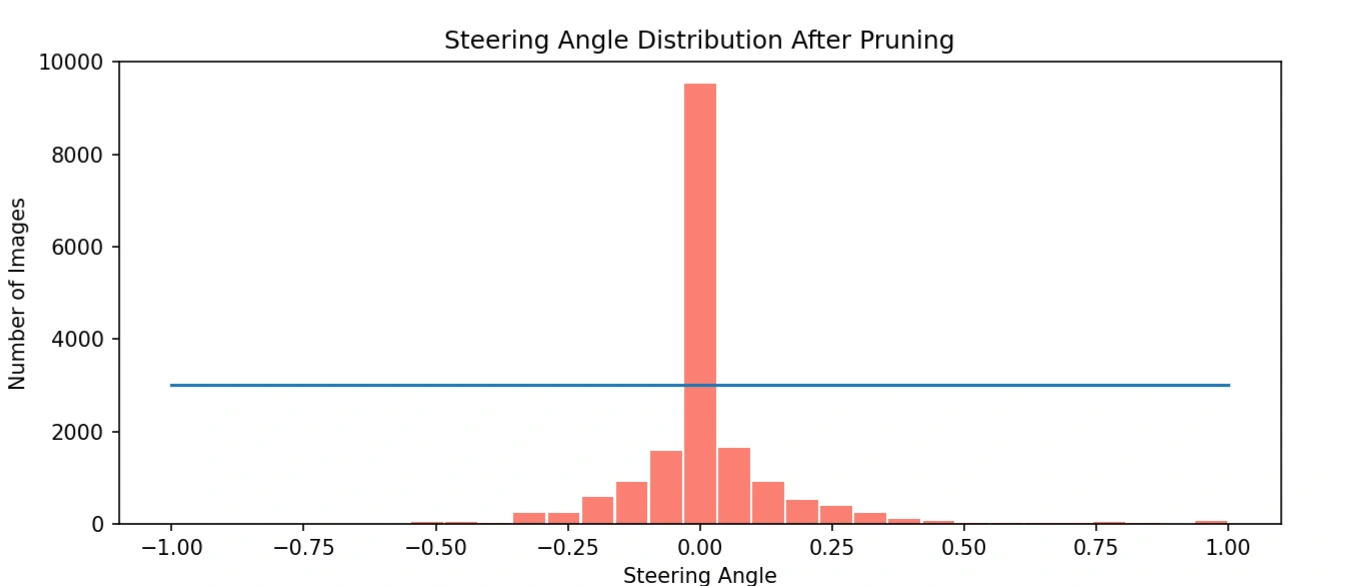
Histogram showing the original steering angle distribution. Notice the sharp spike at 0,
indicating
an overwhelming number of straight-driving samples, which we limit using a
cutoff of 3000.
As the chart shows, our car was trained to drive straight too often. That huge spike in the middle? That’s nearly 10,000+ zero-angle frames—far exceeding all turns combined! If we left it like this, the model would always prefer to go straight, ignoring curves and critical turns.
To fix this, we introduced a cutoff line—limiting each bin to 3000 samples. This
smart pruning keeps the model grounded in real-world driving (where going straight is common), but it
also gives left and right turns the attention they deserve. It’s a balance between reality and
learning diversity.
The horizontal line you see in the histogram? That’s our cutoff threshold, visualized
using:
plt.plot(np.linspace(-1, 1, number_of_bins), [3000] * number_of_bins)Now, with zero-angle samples clipped to 3000 and other bins treated equally, our training data is clean, fair, and ready for the next race!
We’ll use this balanced dataset to train our CNN, teaching it how to navigate lefts, rights, and straights—all with confidence and clarity.
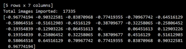
To improve the balance and quality of our training dataset, we implemented a pruning strategy based on steering angle distribution.
Originally, we imported 17,335 images per bin, which showed a heavy skew toward near-zero (straight-driving) steering angles.
This imbalance can cause the model to favor straight paths and underperform on turns and curves.
To address this, we set a cap of 10,805 images per bin, removing 6,530 redundant images per bin.
This process ensures each steering angle range is more equally represented, promoting better generalization and learning across all driving scenarios —
including critical edge cases like sharp turns.
By reducing overrepresented data, we train the model to pay equal attention to both frequent and rare steering behaviors, which ultimately enhances its performance and robustness in real-world environments.
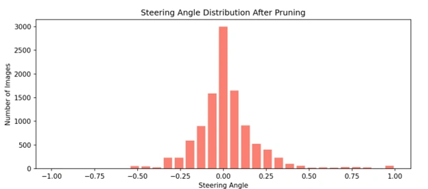
Histogram showing the steering angle distribution after removing redundant data at 3000 cutoff.
Python
        hist_after, bins_after = np.histogram(data['Steering'], nBins)
        plt.figure(figsize=(10, 4))
        plt.bar((bins_after[:-1] + bins_after[1:]) * 0.5, hist_after, width=0.05, color='salmon')
        plt.title('Steering Angle Distribution After Pruning')
        plt.xlabel('Steering Angle')
        plt.ylabel('Number of Images')
        plt.show()
After pruning redundant data from our original dataset, we were left with 10,805 meaningful driving images. To train our self-driving model effectively while preventing overfitting, we divided the data into two key parts:
This splitting process was conducted using the train_test_split() function from Scikit-learn.
By maintaining a fixed random seed, we ensured consistent and reproducible results across experiments.
            CODES:

            xTrain, xVal, yTrain, yVal = train_test_split(imagesPath, steering, test_size=0.2, random_state=5)
            print('Total Traing images: ', len(xTrain))
            print('Total Validation images: ', len(xVal))
This project showcases the application of deep learning to autonomous driving using NVIDIA’s end-to-end Convolutional Neural Network (CNN) architecture. The goal is to predict steering angles from dashcam images, simulating human driving behavior in a car simulator.
We started with thousands of images captured from the car's front-facing camera. The dataset includes center, left, and right images, each paired with a steering angle.
We analyzed the distribution of steering angles to identify potential biases in the dataset. Most angles clustered near zero, indicating straight driving, so we introduced techniques to balance the dataset and improve learning.
No matter how much data you have—it’s never quite enough. When working with limited datasets,
data augmentation becomes your secret weapon. By creatively transforming existing images,
we can unlock thousands of new variations without collecting new data.
Think of it like this: we enhance our dataset by:
These subtle tweaks help our model see the same object from different perspectives,
making it more robust and better at generalization.
📈 For example, starting with 10,000 images, augmentation can boost our dataset to
30,000–40,000 unique training samples—a game-changer for performance and accuracy.
In short, data augmentation lets us train smarter, not harder.
To boost generalization and mimic real-world driving conditions—enabling the model to navigate diverse environments and minimizing overfitting—we applied the following real-time augmentations:
Examples:
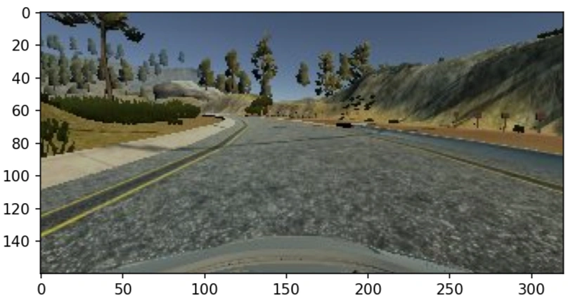
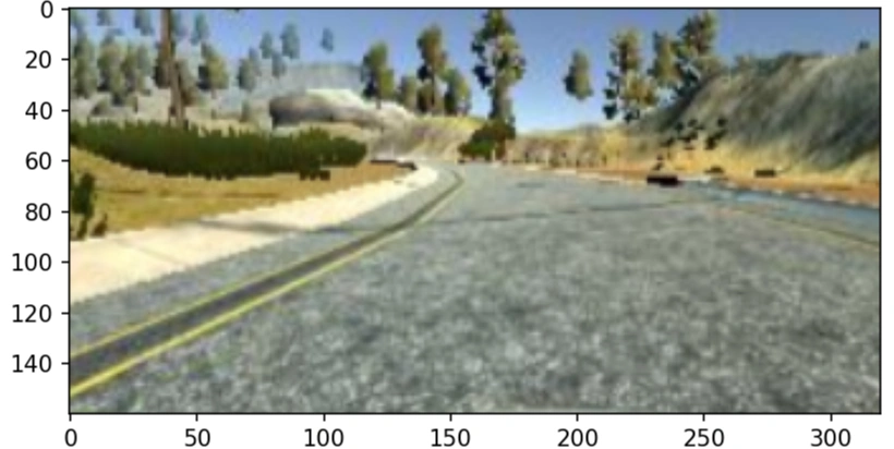
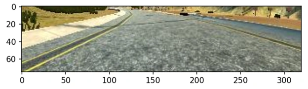
Original Test image
This is the original test image
Changed brightness of image: Adjusting the brightness of images is a powerful augmentation technique that helps the model become resilient to variations in lighting conditions. By randomly increasing or decreasing the brightness of training images, we simulate real-world scenarios such as daytime, dusk, or overcast weather, where the same object may appear lighter or darker. This variety teaches the model to focus on essential features rather than being influenced by lighting intensity, thereby improving its generalization capabilities. In essence, brightness adjustment enhances the model’s robustness and helps reduce overfitting to specific lighting environments.
After changing the brightness of the test image
Zooming image:: Zooming is an effective data augmentation technique that involves scaling an image in or out to simulate how an object might appear at different distances. By applying random zoom transformations during training, we expose the model to various object sizes and perspectives, which helps it learn to recognize patterns regardless of scale. This not only enhances the model's ability to generalize across different real-world scenarios—such as when an object is closer or farther from the camera—but also reduces overfitting by diversifying the training data without needing new images.
After Zooming or resizing the test image
Panned image: Panning involves slightly shifting an image horizontally or vertically—left, right, up, or down—without altering its content. This technique simulates camera movements or changes in object positioning within a frame, helping the model become more robust to spatial variations. By training on panned images, the model learns to recognize objects even when they’re not perfectly centered, which closely mimics real-world conditions where objects can appear anywhere within the frame. This boosts the model’s spatial awareness and improves its performance in dynamic environments.
Panned by moving th test image towards right and upwards.
Flipping image: Flipping, particularly horizontal flipping, mirrors the image by swapping the left and right sides—what appears on the left is shown on the right and vice versa. This augmentation technique is especially useful in scenarios like self-driving car models, where roads, lanes, or objects may appear on either side. By training the model on flipped images, it becomes better equipped to recognize patterns and objects regardless of their orientation, enhancing its ability to generalize and reducing bias toward a specific direction or layout in the dataset.
After horizontally flipped the test image
To increase the diversity of our training dataset and improve the generalization of our self-driving car model, we apply random data augmentation techniques. This randomness ensures that each image may undergo different transformations during each training epoch, making the model more robust.
For each augmentation type (pan, zoom, brightness, or flip), we generate a random number between 0 and 1 using:
  if np.random.rand() < 0.5:
      # Apply specific augmentation
This logic is applied to each augmentation independently. Below is an example of how multiple augmentations can be conditionally applied:
  def augmentImage(img):
      if np.random.rand() < 0.5:
          img = pan(img)

      if np.random.rand() < 0.5:
          img = zoom(img)

      if np.random.rand() < 0.5:
          img = adjustBrightness(img)

      if np.random.rand() < 0.5:
          img = flip(img)

      return img
Each time an image is passed through the augmentImage() function, it may receive:
Because augmentations are decided by independent random checks, their application is dynamic. This produces a wide variety of image versions from a single original.
The augmentation results vary every time the dataset is processed. For example:
This strategy greatly enhances the training dataset without the need for new real-world images. It improves the model’s ability to handle varying lighting, camera angles, and road perspectives—making it much more adaptive and reliable in real-world driving conditions.
Pre-processing is a crucial step to prepare raw images for effective
model training. First, we crop out irrelevant parts of the image—like the sky or the car
hood—to focus on the road. Next, we convert the color space from RGB to YUV, as suggested
by NVIDIA, since YUV better separates brightness from color information, improving
learning efficiency. Gaussian blurring is applied to reduce noise and smooth the image.
We then resize each frame to 200×66 pixels to match the input dimensions
recommended by NVIDIA, optimizing both performance and speed. Finally, normalization by
dividing pixel values by 255 (img/255.0) scales the data to a [0,1] range,
ensuring faster convergence and stable training. Together, these pre-processing techniques
help the model focus on essential visual cues, reduce overfitting, and generalize better to
new driving conditions.
Cropping:
Cropping involves removing unimportant parts of an image—typically the sky or the car hood in driving scenarios—to focus the model’s attention on the most relevant areas, such as the road and surrounding environment. By eliminating these distracting or non-informative regions, cropping helps reduce input noise, improves training efficiency, and enables the model to learn more meaningful features that are critical for accurate decision-making. It also reduces the image size, speeding up computation without losing essential information.
Cropped the test image
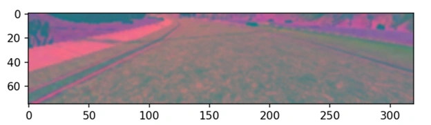
Convert RGB to YUV:
Converting the color space from RGB to YUV separates the image’s brightness (luminance – Y) from its color information (chrominance – U and V). This helps the model focus more effectively on essential structural and lighting details, such as lane lines and road textures, which are better represented in the luminance channel. YUV is especially useful in driving scenarios, as it mimics how humans perceive images—prioritizing brightness over color—thus enhancing the model’s ability to generalize across varying lighting and weather conditions.
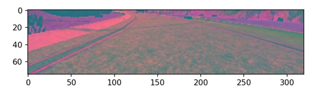
After convertion of RGB to YUV.
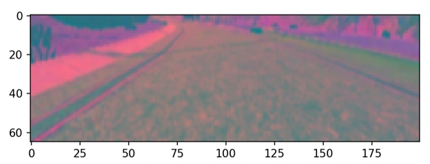
Gaussian Blurring:
Gaussian Blurring smooths the image by reducing high-frequency noise and detail through a weighted average of neighboring pixels. This helps the model by minimizing irrelevant distractions, such as sharp edges or small artifacts, and allows it to focus on the broader, more meaningful patterns and structures—like road shapes, lane lines, and vehicle outlines—thereby improving its ability to learn and generalize from the data.
After blurring the test image
Resizing image to 266x66 pixels:
Resizing the image to 200×66 pixels, as recommended by NVIDIA for end-to-end self-driving models, helps reduce computational load while retaining essential visual features. This lower resolution speeds up training and inference, minimizes memory usage, and forces the model to focus on the most relevant aspects of the scene—like road lanes, vehicles, and obstacles—improving overall performance and efficiency without significant loss of important information.
After resizing the image t0 200x66
Divide image pixels by 255 (IMG/255):
Dividing image pixel values by 255 (img / 255) is a common
normalization technique in image processing that scales the original 0–255 pixel range to a
normalized 0–1 range. Since most images use 8-bit per channel depth, this transformation
ensures that the data fed into the neural network remains consistent and manageable.
Normalization like this improves the model’s training stability by preventing issues such as
exploding or vanishing gradients, which can occur with large input values. It also accelerates
convergence during training by helping the optimizer work more efficiently. Overall, this
step ensures that the model treats all pixel intensities uniformly, which leads to better
learning, improved accuracy, and enhanced overall performance.
After dividing the image pixels by 255 (IMG/255)
In this project, we implemented an efficient batch generator to feed image and steering angle data
into a deep learning model for training a self-driving car. The logic involves reading image paths
and steering angles, deciding whether the model is in training mode, applying real-time data
augmentation if needed, and preprocessing the images before batching them.
The augmentation techniques simulate various driving conditions to improve the model’s robustness.
Preprocessing includes normalization and cropping to remove irrelevant parts of the image (like the
sky or car hood or backgrounds). These steps ensure the model trains on consistent, meaningful data.
Once processed, the images and corresponding steering angles are appended to a batch. This cycle
continues until the batch reaches the desired size, at which point the generator yields the batch to
the training pipeline.
The flow diagram on the right visualizes this process, highlighting the conditional logic and data
transformation steps involved in batch generation for the self-driving car model.
The flow diagram illustrates the logic of the batch generator used in training a self-driving car model. It begins by reading image paths and steering angles. If the model is in training mode, data augmentation and preprocessing steps are applied. Each processed sample is appended to a batch. This process repeats until the batch is full, at which point the batch of images and steering angles is returned for training. This loop ensures efficient, real-time batch preparation with optional augmentation for robust model learning.
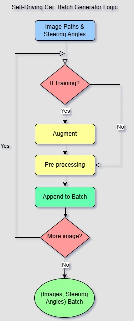
Batch Generation Summary:
CODES:

    def batch_generator(image_paths, steerings, batch_size, train=True):
      while True:
        image_batch = []
        steering_batch = []
        for _ in range(batch_size):
            index = random.randint(0, len(image_paths) - 1)
            if train:
                image, steering = augment_image(image_paths[index], steerings[index])
            else:
                image = load_image(image_paths[index])
                steering = steerings[index]
            image = preprocess_image(image)
            image_batch.append(image)
            steering_batch.append(steering)
        yield np.asarray(image_batch), np.asarray(steering_batch)
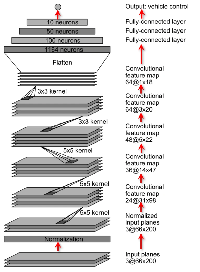
Input Layer:
Input Planes (3@66x200): The model receives RGB images sized 66×200 pixels.
Normalization Layer: This layer scales pixel values to enhance training speed and stability.
Convolutional Layers:
These layers learn spatial features like road edges, curves, and objects, critical for understanding driving environments:
ReLU activations and strided convolutions are used instead of pooling for downsampling.
Flattening & Dense Layers:
The convolutional output is flattened into a 1D vector and passed through fully connected layers:
These layers interpret high-level features to make driving decisions.
Output Layer:
A single neuron outputs the predicted steering angle for the self-driving car.
    Python Codes:


        def createModel():
          # model = Sequential
          model.add(Conv2D(24,(5,5),(2,2), input_shape=(66,200,3), activation='elu' ))
          model.add(Conv2D(36,(5,5),(2,2), activation='elu' ))
          model.add(Conv2D(48,(5,5),(2,2), activation='elu' )) ## SSEE & EXPLAIN INVIDIA flow DIAGRAM
          model.add(Conv2D(64,(3,3), activation='elu' ))
          model.add(Conv2D(64,(3,3), activation='elu' ))

          model.add(Flatten())
          model.add(Dense(100, activation='elu'))
          model.add(Dense(50, activation='elu'))
          model.add(Dense(10, activation='elu'))
          model.add(Dense(1,))

          model.compile(Adam(lr=0.0001), loss='mse')
          return model

        ### RUN THE FUNCTION TO createModel MODEL AS PER NVIDIA Approach
        model = createModel()
        model.summary()
Model Summary Outputs after running the aboves codes:
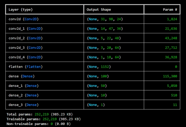
The output image shows: Total params=252,219; Trainable params=252,219; Non-trainable params=0
which are
exactly matching with the recommendation values of NVIDIA.
    Python Codes:


        history = model.fit(batchGen(xTrain, yTrain, 100, 1), steps_per_epoch=300, epochs=60,
            validation_data=batchGen(xVal, yVal, 100,0), validation_steps=200)

        model.save('model.h5')
        print('Model saved')
Model Creation Ecpochs:
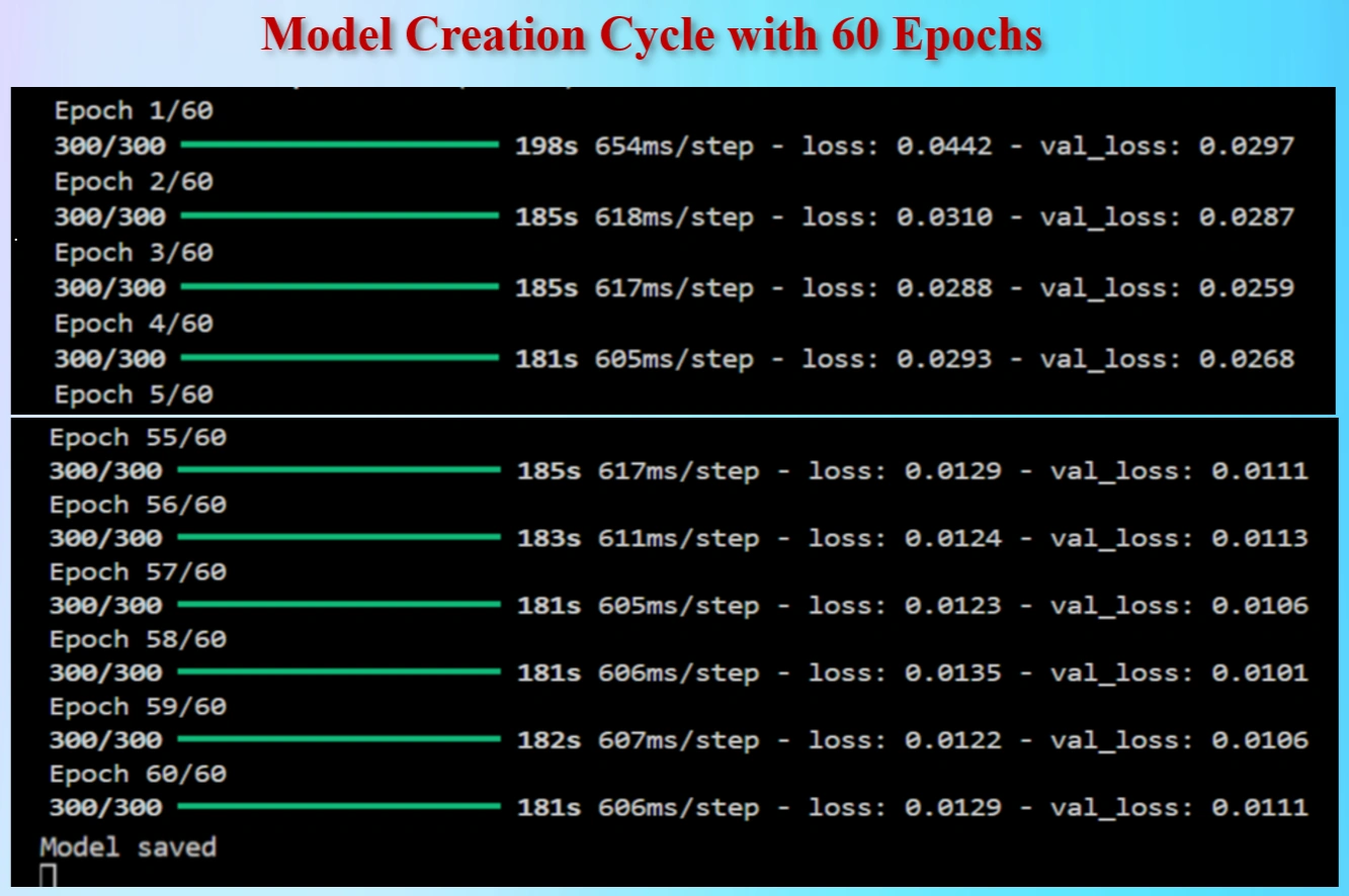
Model created with 60 epochs and saved as "model.h5"
Model created with 60 epochs and saved as "model.h5"
TESTING VIDEO: Driving the trained model on a known track.
VIDEO showing how model running
can run independently after get trained in Udacity Self-Driving Car Simulator.
📹 Video created by HoqueAI during exercise in Udacity Self-Driving Car Simulator.
🎵 Background music: Copyright-free music, china-chinese-asian-music-346568.mp3, from Pixabay.com
VIDEO: Click on the Play Icon to view the video.
My journey into autonomous driving began with a deep interest in applying convolutional neural
networks (CNNs) to real-world problems. I chose to implement NVIDIA's CNN model architecture to
build a self-driving car that could mimic human driving behavior using behavioral cloning.
Despite my early progress, the project soon ran into significant roadblocks due to outdated
dependencies. The Udacity beta simulator was originally built for older versions of Python,
TensorFlow, Keras, and other supporting libraries. As these tools have evolved, compatibility with
the simulator has steadily broken down. Modern Python releases and packages often throw runtime
errors or fail to function entirely with the legacy simulator.
Over the course of several weeks, I invested a great deal of time troubleshooting these issues.
This included creating isolated virtual environments, reinstalling multiple Python versions,
manually adjusting package configurations, and repeatedly rolling back libraries to older states.
Each fix seemed to introduce new bottlenecks, making the development process extremely fragile and
time-consuming.
After much trial and failure runs, I have observed that it gives a little success by making a virtual environment in Python 3.8.0 along with installation of the following older packages:
    pip install Flask==1.1.2
    pip install eventlet==0.30.2
    pip install python-socketio==4.6.1
    pip install numpy==1.22.0
    pip install opencv-python==4.5.5.62
    pip install Pillow==9.0.1
    pip install tensorflow==2.9.1
    pip install Jinja2==3.0.3
    pip install Werkzeug==1.0.1
    pip install itsdangerous==2.0.1
After much difficulty and determination, I finally managed to get the simulator working by
overcoming a range of technical hurdles. But the limitations of this legacy toolset made it clear
that it’s not a sustainable path forward. To truly grow and modernize the project, I’m now
transitioning to CARLA, a powerful open-source simulator that supports the latest
Python packages, advanced sensor simulations, and scalable experimentation in realistic 3D driving
environments.
This transition will help bring my autonomous vehicle experiments closer to real-world
applications, while ensuring compatibility with current and future AI development workflows.
Python codes:
#TO AVOID GPU (Not CPU) WARNINGS
print('Setting Up')
import os
os.environ['TF_CPP_MIN_LOG_LEVEL'] = '3'
from utilis import *
from sklearn.model_selection import train_test_split
import matplotlib.pyplot as plt
import matplotlib.image as mpimg
from imgaug import augmenters as iaa
#### STEP 1
path = 'myData'
data = importDataInfo(path)
#### STEP 2
data = balanceData(data, display=False)
####Step 3
imagesPath, steering = loadData(path, data)
print(imagesPath[0], steering[0])
#### STEP 4 SPLITTING DATA
xTrain, xVal, yTrain, yVal = train_test_split(imagesPath, steering, test_size=0.2, random_state=5)
print('Total Traing images: ', len(xTrain))
print('Total Validation images: ', len(xVal))
##### STEP 5 #####
# images will be augmented during training process
### STEP 6 #### PRE-PROCESSING
## Why pre-processing see transcript
#### STEP 7
### STEP 8 CREATING MODEL AS PER NVIDIA Approach
model = createModel()
model.summary()
#### STEP 9 ######
history = model.fit(batchGen(xTrain, yTrain, 100, 1), steps_per_epoch=100, epochs=10,
validation_data=batchGen(xVal, yVal, 100,1), validation_steps=200)
#### STEP 10 #####
model.save('model.h5')
print('Model saved')
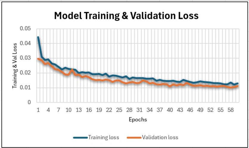
plt.plot(history.history['loss'])
plt.plot(history.history['val_loss'])
plt.legend(['Training', 'Validation'])
plt.ylim([0,1])
plt.title('Loss')
plt.xlabel('Epoch')
plt.show()
Python codes:
      import os
      import eventlet.wsgi
      import socketio
      import eventlet
      import numpy as np
      from flask import Flask

      import tensorflow as tf
      load_model = tf.keras.models.load_model
      import base64
      from io import BytesIO
      from PIL import Image
      from flask import Flask
      import cv2

      model = None  # Declare globally

      sio = socketio.Server()
      app = Flask(__name__)  # __main__
      maxSpeed = 1

      def preProcess(img):
          img = img[60:135, :, :]  # CROPPING THE IMAGE
          img = cv2.cvtColor(img, cv2.COLOR_RGB2YUV)
          img = cv2.GaussianBlur(img, (3, 3), 0)
          img = cv2.resize(img,(200, 65))
          img = img/255
          return img

      @sio.on('telemetry')
      def telemetry(sid, data):
          print("Telemetry received")

          speed = float(data['speed'])
          print("Speed:", speed)

          img_string = data['image']
          print("Image string received")

          image = Image.open(BytesIO(base64.b64decode(img_string)))
          image = np.asarray(image)
          image = preProcess(image)
          image = np.array([image])

          print("Image shape before prediction:", image.shape)

          try:
              steering = float(model.predict(image))
          except Exception as e:
              print("Prediction error:", e)
              steering = 0.0

          throttle = 0.05
          print(f"Steering: {steering}, Throttle: {throttle}, Speed: {speed}")

          send_control(steering, throttle)


      def send_control(steering_angle, throttle):
          sio.emit("steer", data={
              'steering_angle': str(steering_angle),
              'throttle': str(throttle)
          })


      @sio.on('connect')
      def connect(sid, environ):
          print('Connected')
          send_control(0, 0)


      if __name__ == '__main__':
          model = load_model('model.h5')
          #model.summary()  # Optional: check output layer
          app = socketio.Middleware(sio, app)
          eventlet.wsgi.server(eventlet.listen(('', 4567)), app)
Python codes:
      import numpy as np
      import pandas as pd
      import matplotlib.pyplot as plt
      import matplotlib.image as mpimg
      from imgaug import augmenters as iaa
      from sklearn.utils import shuffle
      import os
      import cv2
      import random

      import tensorflow as tf
      model = tf.keras.models.Sequential()
      # Layers
      Conv2D = tf.keras.layers.Conv2D
      Flatten = tf.keras.layers.Flatten
      Dense = tf.keras.layers.Dense
      #control_dependencies = tf.compat.v1.control_dependencies  # tf 2.x way

      # Optimizer
      Adam = tf.keras.optimizers.Adam


      def getName(filePath):
          return filePath.split('\\')[-1]

      def importDataInfo(path):
          columns = ['Center', 'Left', 'Right', 'Steering', 'Throttle', 'Brake', 'Speed']
          data = pd.read_csv(os.path.join(path, 'driving_log.csv'), names = columns)
          #print(data.head())
          #print(data['Center'][0])
          #print(getName(data['Center'][0]))
          data['Center'] = data['Center'].apply(getName)
          #print(data.head())
          print('Total images imported: ', data.shape[0])
          return data


      def balanceData(data, display=True):
          nBins = 31
          samplesPerBin = 1000
          hist, bins = np.histogram(data['Steering'], nBins)
          #print(bins)
          if display:
              center = (bins[:-1] + bins[1:]) * 0.5
              #print(center)
              plt.bar(center, hist, width = 0.06)
              plt.plot((-1,1), (samplesPerBin, samplesPerBin))
              plt.show()

          #REMOVE REDUNDENT DATA
          removeIndexList = []
          for j in range(nBins):
              binDataList = []
              for i in range(len(data['Steering'])):
                  if data['Steering'][i] >= bins[j] and data['Steering'][i] <= bins[j+1]:
                      binDataList.append(i)
              binDataList = shuffle(binDataList)
              binDataList = binDataList[samplesPerBin:]
              removeIndexList.extend(binDataList)
          print('Removed images: ', len(removeIndexList))
          data.drop(data.index[removeIndexList], inplace = True)
          print('Remaining images: ', len(data))

          if display:
              hist, _ = np.histogram(data['Steering'], nBins)
              plt.bar(center, hist, width = 0.06)
              plt.plot((-1,1), (samplesPerBin, samplesPerBin))
              plt.show()

          return data

      def loadData(path, data):
          imagesPath = []
          steering = []

          for i in range(len(data)):
              indexedData = data.iloc[i]
              #print(indexedData)
              imagesPath.append(os.path.join(path, 'IMG', indexedData[0]))
              #print(os.path.join(path, 'IMG', indexedData[0]))
              steering.append(float(indexedData[3]))

          imagesPath = np.array(imagesPath)
          steering = np.array(steering)
          return imagesPath, steering

      def augmentImage(imgPath, steering):
          img = mpimg.imread(imgPath)
          #print(np.random.rand(), np.random.rand(), np.random.rand(), np.random.rand(), np.random.rand())
          ## PAN
          if np.random.rand() < 0.5:
              pan = iaa.Affine(translate_percent={'x':(-0.1,0.1), 'y':(-0.1,0.1)})
              img = pan.augment_image(img)

          #### ZOOM
          if np.random.rand() < 0.5:
              zoom = iaa.Affine(scale=(1,1.3))
              img = zoom.augment_image(img)

          #### BRIGHTNESS
          if np.random.rand() < 0.5:
              brightness = iaa.Multiply((0.4, 1.2)) # This is a tuple, meaning: randomly multiply pixel values by any value in [0.4, 1.2]
              img = brightness.augment_image(img)

          #### FLIP ####
          if np.random.rand() < 0.5:
              img = cv2.flip(img, 1)
              steering = -steering

          return img, steering

      # imgRe, st = augmentImage('test.jpg', 0)
      # plt.imshow(imgRe)
      # plt.show()

      def preProcessing(img):
          img = img[60:135, :, :]  # CROPPING THE IMAGE
          img = cv2.cvtColor(img, cv2.COLOR_RGB2YUV)
          img = cv2.GaussianBlur(img, (3,3),0)
          img = cv2.resize(img,(200, 65))
          img = img/255
          return img

      imgRe = preProcessing( mpimg.imread('test.jpg'))
      plt.imshow(imgRe)
      plt.show()

      def batchGen(imagesPath, steeringList, batchSize, trainFlag):
          while True:
              imgBatch = []
              steeringBatch = []
              for i in range(batchSize):    ### FOR 1 image
                  index = random.randint(0, len(imagesPath)-1)
                  if trainFlag:
                      img, steering =  augmentImage(imagesPath[index], steeringList[index])
                  else:
                      img = mpimg.imread(imagesPath[index])
                      steering = steeringList[IndexError]

                  img = preProcessing(img)
                  imgBatch.append(img)
                  steeringBatch.append(steering)

              yield (np.asarray(imgBatch), np.asarray(steeringBatch))

      def createModel():
      # model = Sequential
          model.add(Conv2D(24,(5,5),(2,2), input_shape=(66,200,3), activation='elu' ))
          model.add(Conv2D(36,(5,5),(2,2), activation='elu' ))
          model.add(Conv2D(48,(5,5),(2,2), activation='elu' )) ## SSEE & EXPLAIN INVIDIA flow DIAGRAM
          model.add(Conv2D(64,(3,3), activation='elu' ))
          model.add(Conv2D(64,(3,3), activation='elu' ))

          model.add(Flatten())
          model.add(Dense(100, activation='elu'))
          model.add(Dense(50, activation='elu'))
          model.add(Dense(10, activation='elu'))
          model.add(Dense(1,))

          model.compile(Adam(lr=0.0001), loss='mse')
          return model
Following NVIDIA’s architecture, the model consists of:
model.save('nvidia_self_driving_model.h5')plt.plot(history.history['loss'])
plt.plot(history.history['val_loss'])
plt.legend(['Training Loss', 'Validation Loss'])
plt.title('Loss Over Epochs')
plt.xlabel('Epoch')
plt.ylabel('MSE Loss')
plt.show()A deep learning model was built using TensorFlow + Keras based on NVIDIA’s end-to-end self-driving car design.
nvidia_self_driving_model.h5Loss graphs were generated to evaluate model learning progress:
plt.plot(history.history['loss'])
plt.plot(history.history['val_loss'])
plt.legend(['Training Loss', 'Validation Loss'])
plt.title('Loss Over Epochs')
plt.xlabel('Epoch')
plt.ylabel('MSE Loss')
plt.show()Also, TensorFlow logs were suppressed for cleaner outputs:
import os
os.environ['TF_CPP_MIN_LOG_LEVEL'] = '3'This custom generator dynamically loads and augments training data to optimize memory usage and training quality.
def batch_generator(image_paths, steerings, batch_size, train=True):
      while True:
          image_batch = []
          steering_batch = []
          for _ in range(batch_size):
              index = random.randint(0, len(image_paths) - 1)
              if train:
                  image, steering = augment_image(image_paths[index], steerings[index])
              else:
                  image = load_image(image_paths[index])
                  steering = steerings[index]
              image = preprocess_image(image)
              image_batch.append(image)
              steering_batch.append(steering)
yield np.asarray(image_batch), np.asarray(steering_batch)💡 If you liked this project, stay tuned for more AI experiments!