
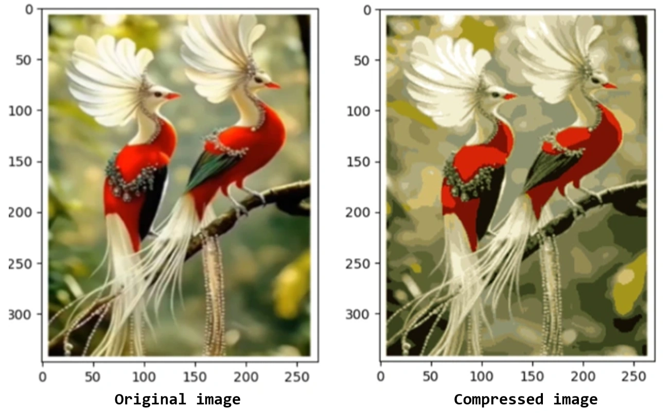
Image 1: Comparison between original and Compressed images of red_birds
This project presents a concise yet powerful application of K-Means Clustering and Principal Component Analysis (PCA) to explore image compression and alpha channel transparency in digital images.
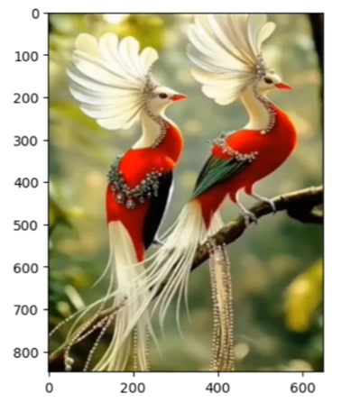
Image 2: Original picture of a bird before compression
In this project, we explore two fundamental machine learning techniques: K-Means Clustering and Principal Component Analysis (PCA). These techniques are widely used in image compression, data compression, pattern recognition, and computer vision. Through practical examples, we demonstrate how clustering helps reduce complexity in images and how dimensionality reduction preserves essential features while simplifying data representation.
K-Means Clustering is an unsupervised learning algorithm used to group similar data points into K clusters. K-means clustering is the Process in clustering similar data points in a 2D space into groups and widely used in grouping like:
In the context of image processing, we apply K-Means to perform color quantization, reducing the number of colors in an image while maintaining visual integrity.
The goal of K-Means is to minimize the total within-cluster variance, also known as the cost function (J):
\[ J = \sum_{i=1}^{m} \sum_{k=1}^{K} w_{ik} || x_i - C_k ||^2 \]
where:
Centroid is the center of a cluster. It is an imaginary point that represents the average position of all points in that cluster.
The centroid of a cluster \( k \) is calculated as the mean of all points \( x_i \) in that cluster:
\[ C_k = \frac{1}{N_k} \sum_{i=1}^{N_k} x_i \]
where:
Principal Component Analysis (PCA) is a powerful dimensionality reduction technique that finds the most important features in high-dimensional data. PCA is particularly useful in face recognition, where we extract key facial features to represent images efficiently.
How We Proceed
Project Goals
Through these examples, we highlight the power of unsupervised learning techniques in image processing and data compression. Let’s dive in! 🚀
1.1 Importing Required Libraries:
            Python:

            import imageio.v2 as imageio
            import matplotlib.pyplot as plt
            import numpy as np
            from random import sample #Used for random initialization
Exppanation:
numpy is used for numerical operations, especially handling matrices and arrays.matplotlib.pyplot is used for visualization.random.sample helps in randomly selecting data points for initialization.1.2 Function to Compute Squared Distance
            Python:

            def distSquared(point1, point2):
                assert point1.shape == point2.shape
                return np.sum(np.square(point2 - point1))
def distSquared(point1, point2) computes the squared Euclidean distance between two points.1.3 Finding Closest Centroids
Python codes:
            Python:

            def findClosestCentroids(myX, mycentroids):
                idxs = np.zeros((myX.shape[0], 1))

                for x in range(idxs.shape[0]):
                    mypoint = myX[x]
                    mindist, idx = 9999999, 0  # Initialize with a large number

                    for i in range(mycentroids.shape[0]):
                        mycentroid = mycentroids[i]
                        distsquared = distSquared(mycentroid, mypoint)

                        if distsquared < mindist:
                            mindist = distsquared
                            idx = i

                    idxs[x] = idx  # Assign closest centroid index

                return idxs
def findClosestCentroids(myX, mycentroids) assigns each data point in X to the nearest centroid.1.4 Assigning Data Points to Clusters
            Python:

                idxs = findClosestCentroids(X, initial_centroids)
                print(idxs[:3].flatten())  # Print the first 3 cluster assignments

                Output:
                    [0. 2. 1.]
findClosestCentroids is called with X (data points) and initial_centroids (three predefined centroids).1.5 Computing New Centroid Positions
            Python:

                def computeCentroids(myX, myidxs):
                    """
                    Function takes in the X matrix and the index vector
                    and computes a new centroid matrix.
                    """
                    subX = []
                    for x in range(len(np.unique(myidxs))):
                        subX.append(np.array([myX[i] for i in range(myX.shape[0]) if myidxs[i] == x]))

                    return np.array([np.mean(thisX,axis=0) for thisX in subX])
def computeCentroids(myX, myidxs) computes the new centroid positions after assigning data points to clusters.
myX: The dataset (each row is a data point).myidxs: The cluster assignments for each point (from findClosestCentroids).1.6 Finding Closest Centroids
Python codes:
            Python:

                def runKMeans(myX, initial_centroids, K, n_iter):
                    """
                    Function that actually does the iterations
                    """
                    centroid_history = []
                    current_centroids = initial_centroids

                    for myiter in range(n_iter):
                        centroid_history.append(current_centroids)
                        idxs = findClosestCentroids(myX, current_centroids)
                        current_centroids = computeCentroids(myX, idxs)

                    return idxs, centroid_history
def runKMeans(myX, initial_centroids, K, n_iter) implements the iterative K-means clustering process.myX: The dataset.initial_centroids: Initial centroid positions.K: Number of clusters.n_iter: Number of iterations for K-means.centroid_history.findClosestCentroids).computeCentroids).Why is this Needed?
centroid_history allows visualization of centroid movement.1.7 How Initial Centroids Affect K-Means Clustering Visualizations?
            Python:

                def chooseKRandomCentroids(myX, K):
                    rand_indices = sample(range(0,myX.shape[0]),K)
                    return np.array([myX[i] for i in rand_indices])
Explanation
def chooseKRandomCentroids(myX, K) selects K random points from
the dataset X to use as initial centroids for K-Means clustering.sample(range(0,myX.shape[0]),K) randomly selects K unique indices from the dataset.🛠 Why is this needed?
What is Alpha Channel?
An alpha channel is an additional layer in an image that controls transparency. It is mainly used in RGBA images, where:
A fully opaque pixel has an alpha value of 255, while a fully transparent pixel has an alpha value of 0.
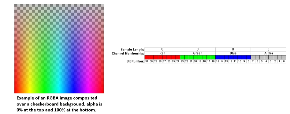
Image 3: K-means Clustering graph 3 with different initial Centroids
Why Remove the Alpha Channel Before Image Compression?
When performing K-Means clustering for image compression, removing the alpha channel is necessary due to the following reasons:
- The clustering algorithm groups colors (R, G, B), not transparency levels.
- If the alpha channel is included, K-Means would treat transparent and opaque pixels as different colors, leading to inaccurate clustering.
- Many image processing functions expect a 3-channel (RGB) image and do not support 4-channel (RGBA) images.
- Including the alpha channel may cause errors or unexpected results.
- Removing the alpha channel ensures that all pixels have the same structure (R, G, B values only).
- This simplifies reshaping and processing the image for compression.
How Do We Remove the Alpha Channel?
In our code, we check if the image has an alpha channel and remove it:
                        # Check if the image has an alpha channel (RGBA format)
                        if A.shape[2] == 4:
                            A = A[:, :, :3]  # Keep only the first three channels (RGB)
✅ This keeps only the first 3 channels (R, G, B) and discards transparency.
When is the Alpha Channel Needed?
While removing the alpha channel is essential for K-Means clustering, it is useful in other cases like:
For image compression, removing the alpha channel helps produce a clean and accurate color clustering.
2.2 K-means on pixels:
This part of the project applies K-Means clustering to an image to perform image compression by reducing the number of unique colors in the image.
Python codes:
            # Load image
            datafile = r'd:\mysite\images\red_birds2.png'
            A = imageio.imread(datafile)

            # Check if image has 4 channels (RGBA), convert to RGB
            if A.shape[2] == 4:  # Check if there's an alpha channel
                A = A[:, :, :3]  # Keep only the first three channels (RGB)

            # Display shape and image
            print("A shape after removing alpha channel:", A.shape)
            plt.imshow(A)
            plt.axis("off")  # Hide axes
            plt.show()

            A = A / 255.0     # Normalize pixel values (0 to 1)
            A = A.reshape(-1, 3) # Reshape image to (num_pixels, 3)
            print("New A shape:", A.shape)

            # Run k-means clustering
            myK = 16
            idxs, centroid_history = runKMeans(A, chooseKRandomCentroids(A, myK), myK, n_iter=10)
Comments:
In the codes by myK = 16, we explicitly set 16 centroids enabling to
store 16 colors in the future.
Output:
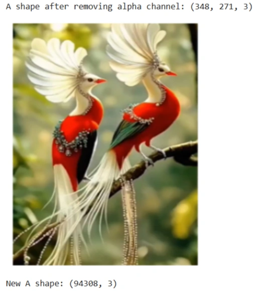
Image 4: Bird image for compression after removing alpha channel
The output indicates that now the image is of (348, 271, 3), which means image is:
At the bottom of output image "New A shape: (94308, 3)" indicates that:
Assigning Each Pixel to the Closest Centroid
            Python:

                idxs = findClosestCentroids(A, centroid_history[-1])
What this does:
centroid_history[-1] contains the final centroid positions after 10 iterations of K-Means.idxs stores the index of the closest centroid for each pixel in the reshaped image.✅ At this point, each pixel is mapped to one of the 16 colors from K-Means clustering.
Reconstructing the Image with 16 Colors
            final_centroids = centroid_history[-1]

            final_image = np.zeros((idxs.shape[0], 3))  # Create new image with only 16 colors

            for x in range(final_image.shape[0]):
                final_image[x] = final_centroids[int(idxs[x].item())]  # ✅ Use .item() to extract scalar
What this does:
final_centroids = centroid_history[-1] → Stores the final 16 centroid colors.final_image = np.zeros((idxs.shape[0], 3)) → Creates an empty array for
the compressed image.final_image to the corresponding centroid
color.✅ At this point, the image is reconstructed using only 16 unique colors instead of the original full-color spectrum.
Displaying the Images
            orig_height, orig_width = 348, 271  # Use the correct values
                # Get the original image dimensions
            plt.figure()  # Reshape the original and compressed images correctly
            dummy = plt.imshow(A.reshape(orig_height, orig_width, 3))  # ✅ Correct shape
            plt.figure()
            dummy = plt.imshow(final_image.reshape(orig_height, orig_width, 3))  # ✅ Correct shape
            plt.show()
What this does:
plt.figure() and plt.imshow(A.reshape(orig_height, orig_width, 3))plt.figure() and plt.imshow(final_image.reshape(orig_height, orig_width, 3))plt.show() → Renders both images.✅ At this point, two images are displayed as output:
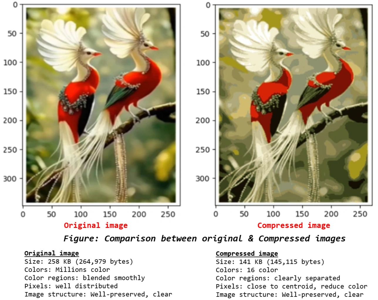
Image 5: Comparison between original and compressed image.
Observations
While compression significantly reduces the number of unique colors in the image, it does not degrade the overall quality. Instead, it enhances the separation of different regions, making boundaries between colors more visible.
Key Takeaways:
- PCA was applied to image data, starting with feature normalization and computing
Singular Value Decomposition (SVD) to extract principal components.
- This helped project high-dimensional image data into lower-dimensional spaces while
retaining important features.
- By extracting eigenfaces from a dataset of human faces, we visualized the most significant
facial features.
- Reducing image dimensions allowed us to compress and reconstruct faces while analyzing
how much detail was preserved.
- Images were projected onto a lower-dimensional subspace (e.g., 36 principal components) and
reconstructed to evaluate the loss of detail.
- The reconstructed images retained main features, demonstrating PCA’s effectiveness in
image compression.
- PCA was used to reduce RGB color data from 3D to 2D for easier visualization of color clusters.
- The final PCA projection plot illustrated how PCA can assist in image segmentation
and clustering.
This project successfully demonstrated PCA’s power in reducing data complexity while maintaining essential structure in images. From face recognition to color compression, PCA proves to be a valuable tool in machine learning and computer vision.
Future improvements could involve exploring non-linear dimensionality reduction techniques like t-SNE or Autoencoders for better visualization and reconstruction quality.
🚀 Thank you for following along!
I sincerely thank Prof. Andrew NG (DeepLearning.AI, Stanford University) for his inspiring courses that laid the foundation for this project.
 www.HoqueAi.com