

AI Generated image: Feature Learning in Neural Networks
This project explores the inner workings of neural networks, focusing on how features are learned and visualized during training using handwritten digit datasets.
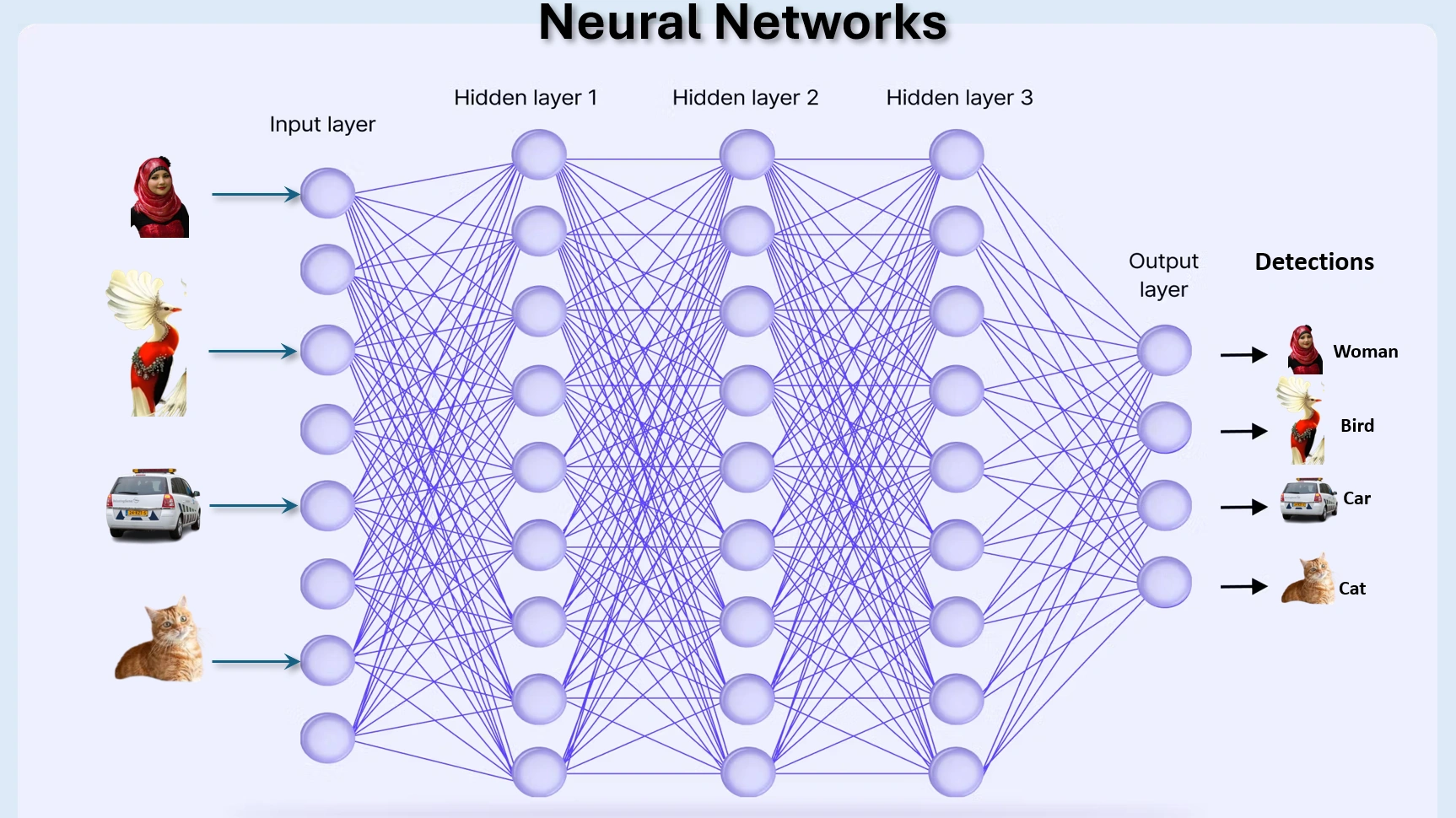
Image 1: Neural Network layers
Neural networks are often seen as "black boxes", but what really happens
inside them? This project, "Inside the Neural Network: Feature Learning & Visualization",
explores how neural networks process and transform input data at hidden layers. Our focus is
to visualize the intermediate representations learned by the network,
providing an intuitive understanding of how deep learning models recognize patterns.
Through structured exercises, we train a neural network on handwritten digits and analyze
how the hidden layers extract and refine features from raw input. By the
end of the project, we generate visualizations from a hidden layer to observe how the
network interprets and distinguishes different digit structures. This approach makes
abstract concepts more tangible, offering both an educational and engaging perspective
on deep learning.
Let’s dive in and uncover the hidden intelligence of neural networks! 🚀
In this project our aims are to implement a neural network model to classify handwritten digits (0-9).
Run the following codes:
            %matplotlib inline
            import numpy as np
            import matplotlib.pyplot as plt
            import pandas as pd
            import scipy.io #Used to load the OCTAVE *.mat files
            import scipy.misc #Used to show matrix as an image
            import matplotlib.cm as cm #Used to display images in a specific colormap
            import random #To pick random images to display
            import scipy.optimize #fmin_cg to train neural network
            import itertools
            from scipy.special import expit #Vectorized sigmoid function

            datafile = r'd:\mlprojects\data\ex4data1.mat'
            #mat = scipy.io.loadmat( datafile )

            mat = scipy.io.loadmat(datafile, squeeze_me=True)
            print(mat.keys())
            X, y = mat['X'], mat['y']

            X, y = mat['X'], mat['y']
            #Insert a column of 1's to X as usual
            X = np.insert(X,0,1,axis=1)
            print("'y' shape: %s. Unique elements in y: %s"%(mat['y'].shape,np.unique(mat['y'])))
            print("'X' shape: %s. X[0] shape: %s"%(X.shape,X[0].shape))
            #X is 5000 images. Each image is a row. Each image has 400 pixels unrolled (20x20)
            #y is a classification for each image. 1-10, where "10" is the handwritten "0"
Outputs: After running the above codes:
        dict_keys(['__header__', '__version__', '__globals__', 'X', 'y'])
        'y' shape: (5000,). Unique elements in y: [ 1  2  3  4  5  6  7  8  9 10]
        'X' shape: (5000, 401). X[0] shape: (401,)
1. Code Breakdown:
%matplotlib inline: Ensures that plots are displayed within the notebook.numpy, matplotlib.pyplot, pandas: Commonly used Python libraries for numerical
computation and data visualization.scipy.io: Used to load .mat (MATLAB) files.scipy.misc: Used for image display. However, scipy.misc.toimage is
deprecated in recent versions.random: Helps select random images.scipy.optimize: Used for optimization tasks such as training a neural network.itertools: Provides efficient looping constructs.scipy.special.expit: Implements a vectorized
sigmoid function (alternative to manually defining sigmoid(x)).Loading ex4data1.mat:
.mat file.scipy.io.loadmat() function loads the data into a Python dictionary.squeeze_me=True ensures that unnecessary dimensions are removed.Extracting X and y:
X: Represents the feature matrix (5000 handwritten digit images). Each image is 20×20 pixels, stored as a row of 400 values.y: Represents the labels (digits 1 to 10, where 10 corresponds to digit ‘0’).Adding a Bias Column to X:
X for bias (intercept term).
This is required for neural network computations.Output Analysis
a) 'dict_keys(...)': The dataset contains five keys:
'X': Feature matrix of shape (5000, 400).'y': Labels corresponding to the 5000 images.'__header__', '__version__', '__globals__': Metadata information.b) 'y' shape: (5000,) confirms that there are 5000 labels.
c) 'X' shape: (5000, 401)':
(5000, 401).Run the following codes in Jupyter Notebook cells:
            from PIL import Image  # Import Pillow

            def getDatumImg(row):
                """
                Function that is handed a single np array with shape 1x400,
                crates an image object from it, and returns it
                """
                width, height = 20, 20
                square = row[1:].reshape(width,height)
                return square.T

            def displayData(indices_to_display=None):
            """
                Function that picks 100 random rows from X, creates a 20x20 image from each,
                then stitches them together into a 10x10 grid of images, and shows it.
                """
                width, height = 20, 20
                nrows, ncols = 10, 10
                if not indices_to_display:
                    indices_to_display = random.sample(range(X.shape[0]), nrows * ncols)

                big_picture = np.zeros((height * nrows, width * ncols))

                irow, icol = 0, 0
                for idx in indices_to_display:
                    if icol == ncols:
                        irow += 1
                        icol = 0
                    iimg = getDatumImg(X[idx])
                    big_picture[irow * height : irow * height + iimg.shape[0], icol * width : icol * width + iimg.shape[1]] = iimg
                    icol += 1

            fig = plt.figure(figsize=(6, 6))
            big_picture = (big_picture - big_picture.min()) / (big_picture.max() - big_picture.min()) * 255  # Normalize to 0-255
            img = Image.fromarray(big_picture.astype(np.uint8))  # Convert to 8-bit image
            plt.imshow(img, cmap=cm.Greys_r)
            plt.axis("off")  # Hide axes for better visualization
            plt.show()

        displayData()
Output: after running the codes displayed handwritten image.
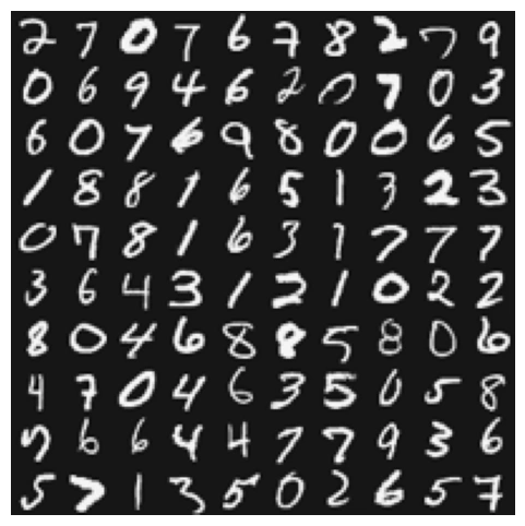
Image 2: Hanwritten digits
                datafile = r'd:\mlprojects\data\ex4weights.mat'
                mat = scipy.io.loadmat(datafile)
                Theta1, Theta2 = mat['Theta1'], mat['Theta2']
.mat file.Theta1 and Theta2 are weight matrices for the two
layers in a neural network.Theta1 has dimensions (25, 401), corresponding to
25 hidden units and 400 input features + bias.Theta2 has dimensions (10, 26), corresponding to
10 output units and 25 hidden units + bias.Analyse the following codes:
            input_layer_size = 400
            hidden_layer_size = 25
            output_layer_size = 10
            n_training_samples = X.shape[0]
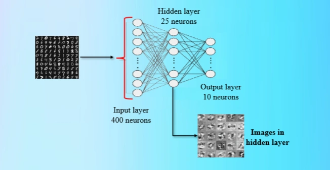
Image 3: Neuron Network parameters
The neural network consists of:
The number of training samples is taken from X.shape[0] (5000 images).
Utility Functions for Reshaping Matrices
Run codes
            def flattenParams(thetas_list):
                flattened_list = [ mytheta.flatten() for mytheta in thetas_list ]
                combined = list(itertools.chain.from_iterable(flattened_list))
                return np.array(combined).reshape((len(combined),1))

            def reshapeParams(flattened_array):
                theta1 = flattened_array[:(input_layer_size+1)*hidden_layer_size] \
                        .reshape((hidden_layer_size,input_layer_size+1))
                theta2 = flattened_array[(input_layer_size+1)*hidden_layer_size:] \
                        .reshape((output_layer_size,hidden_layer_size+1))
                return [ theta1, theta2 ]

            def flattenX(myX):
                return np.array(myX.flatten()).reshape((n_training_samples*(input_layer_size+1),1))

            def reshapeX(flattenedX):
                return np.array(flattenedX).reshape((n_training_samples,input_layer_size+1))
Code Explanation
flattenParams(): Converts multiple matrices (Theta1, Theta2)
into a single vector for optimization.reshapeParams(): Converts the flattened vector back into Theta1 and
Theta2 with the correct dimensions.Cost Function for Neural Network
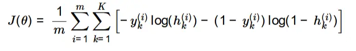
The cost function for the neural network is defined as:
Cost Function Formula:
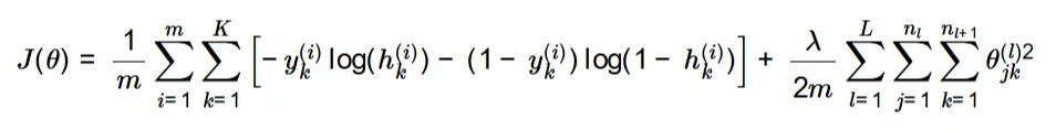
where:
The regularization term is included to penalize large weights and avoid overfitting.
            def computeCost(mythetas_flattened,myX_flattened,myy,mylambda=0.):
                mythetas = reshapeParams(mythetas_flattened)
                myX = reshapeX(myX_flattened)

                total_cost = 0.
                m = n_training_samples

                for irow in range(m):
                    myrow = myX[irow]
                    myhs = propagateForward(myrow,mythetas)[-1][1] # Hypothesis

                    tmpy  = np.zeros((10,1))
                    tmpy[myy[irow]-1] = 1  # One-hot encoding

                    mycost = -tmpy.T.dot(np.log(myhs))-(1-tmpy.T).dot(np.log(1-myhs))
                    total_cost += mycost

                total_cost = float(total_cost) / m  # Normalize

                # Compute the regularization term
                total_reg = 0.
                for mytheta in mythetas:
                    total_reg += np.sum(mytheta*mytheta) #element-wise multiplication
                total_reg *= float(mylambda)/(2*m)

                return total_cost + total_reg
y into a 10×1 vector.Feedforward Propagation
            def propagateForward(row,Thetas):
                features = row
                zs_as_per_layer = []
                for i in range(len(Thetas)):
                    Theta = Thetas[i]
                    z = Theta.dot(features).reshape((Theta.shape[0],1))
                    a = expit(z) # Sigmoid Activation
                    zs_as_per_layer.append((z, a))

                    if i == len(Thetas)-1:
                        return zs_as_per_layer

                    a = np.insert(a,0,1) # Add bias unit
                    features = a
z (weighted sum) and a (activation).The final output layer predicts a probability distribution over 10 classes.
Feedforward:
Feedforward is the process in which input data moves through a neural network, layer by layer, to produce an output. Each neuron applies a weighted sum of its inputs, followed by an activation function (like the sigmoid function), to generate activations that are passed to the next layer. This process continues until the final output layer is reached. Feedforward is used during both training and prediction to compute the output of the network.
Cost function:
The cost function measures how well the neural network's predicted outputs match the actual labels. It quantifies the error between the predicted and actual values. In classification problems, a common cost function is the cross-entropy loss. A lower cost indicates a better-performing model. Regularization (like adding a penalty term for large weights) is often used to prevent overfitting.
Backpropagation:
Backpropagation (short for "backward propagation of errors") is the method used to train a neural network by updating its weights to minimize the cost function. It involves computing the gradient of the cost function with respect to each weight using the chain rule of calculus. The gradients are then used to adjust the weights in the opposite direction of the error, ensuring the network improves over multiple iterations. This process continues until the cost function converges to a minimum.
Feedforward and Backpropagation in Neural Networks
1. Feedforward and Cost Function
1.1 Cost Function (Without Regularization)
The cost function for the neural network is defined as:
Cost Function Formula:
Code used:
            myThetas = [ Theta1, Theta2 ]
            print(computeCost(flattenParams(myThetas),flattenX(X),y))

            Output:
            0.2876
Running the cost function without regularization gives a cost of **0.2876**.
1.2 Cost Function (With Regularization)
To prevent overfitting, a regularization term is added:
Formula:
With regularization (\(\lambda=1\)), the cost is **0.3845**.
Computed the cost function with an added regularization term to prevent overfitting.
Key Steps:
mylambda=1.0 is passed to computeCost, enabling regularization.computeCost calculates and prints the cost with regularization.2. Backpropagation
2.1 Sigmoid Gradient
Computed the gradient of the sigmoid function, which is essential for backpropagation.
Formula:
\[ g'(z) = \sigma(z) (1 - \sigma(z)) \]
We have the following function in the code:
            def sigmoidGradient(z):
                dummy = expit(z)
                return dummy*(1-dummy)
Key steps:
expit(z) function computes the sigmoid function.σ(z)
by 1 - σ(z).2.2 Random Initialization
Initializes the neural network weights randomly in a small range to avoid symmetry in learning. The weights are initialized in the range:
\[ -\epsilon \leq \theta \leq \epsilon \]
where \(\epsilon = 0.12\).
Used genRandThetas() function in codes
            def genRandThetas():
                epsilon_init = 0.12
                theta1_shape = (hidden_layer_size, input_layer_size+1)
                theta2_shape = (output_layer_size, hidden_layer_size+1)
                rand_thetas = [ np.random.rand( *theta1_shape ) * 2 * epsilon_init - epsilon_init, \
                                np.random.rand( *theta2_shape ) * 2 * epsilon_init - epsilon_init]
                return rand_thetas
Key Steps:
epsilon_init = 0.12 is used as the range for random initialization.theta1 and theta2) are created for
the hidden and output layers.[-ε, ε] using
NumPy’s np.random.rand().2.3 Backpropagation Algorithm
Purpose:Implements the backpropagation algorithm to compute the gradients needed for weight updates.
            def backPropagate(mythetas_flattened,myX_flattened,myy,mylambda=0.):

                # First unroll the parameters
                mythetas = reshapeParams(mythetas_flattened)

                # Now unroll X
                myX = reshapeX(myX_flattened)

                #Note: the Delta matrices should include the bias unit
                #The Delta matrices have the same shape as the theta matrices
                Delta1 = np.zeros((hidden_layer_size,input_layer_size+1))
                Delta2 = np.zeros((output_layer_size,hidden_layer_size+1))

                # Loop over the training points (rows in myX, already contain bias unit)
                m = n_training_samples
                for irow in range(m):
                    myrow = myX[irow]
                    a1 = myrow.reshape((input_layer_size+1,1))
                    # propagateForward returns (zs, activations) for each layer excluding the input layer
                    temp = propagateForward(myrow,mythetas)
                    z2 = temp[0][0]
                    a2 = temp[0][1]
                    z3 = temp[1][0]
                    a3 = temp[1][1]
                    tmpy = np.zeros((10,1))
                    tmpy[myy[irow]-1] = 1
                    delta3 = a3 - tmpy
                    delta2 = mythetas[1].T[1:,:].dot(delta3)*sigmoidGradient(z2) #remove 0th element
                    a2 = np.insert(a2,0,1,axis=0)
                    Delta1 += delta2.dot(a1.T) #(25,1)x(1,401) = (25,401) (correct)
                    Delta2 += delta3.dot(a2.T) #(10,1)x(1,25) = (10,25) (should be 10,26)

                D1 = Delta1/float(m)
                D2 = Delta2/float(m)

                #Regularization:
                D1[:,1:] = D1[:,1:] + (float(mylambda)/m)*mythetas[0][:,1:]
                D2[:,1:] = D2[:,1:] + (float(mylambda)/m)*mythetas[1][:,1:]

                return flattenParams([D1, D2]).flatten()
Key Steps:
mythetas_flattened
and myX_flattened are reshaped to their original forms.Delta1 and Delta2
(accumulators for weight updates) are set to zero.(delta3) is calculated as the difference between
predicted and actual output.(delta2) is computed using the sigmoid gradient.Delta1 and Delta2.The computed gradients are then used to update the weights in gradient descent.
2.4 Backpropagation and Gradient Checking
Computing Gradients for Backpropagation
            #Compute D matrices for the Thetas provided
            flattenedD1D2 = backPropagate(flattenParams(myThetas),flattenX(X),y,mylambda=0.)
            D1, D2 = reshapeParams(flattenedD1D2)
Key Steps:
backPropagate() to compute the gradients of the cost function using backpropagation.flattenParams(myThetas) ensures that the parameter matrices are flattened into
a single vector before passing them to the function.reshapeParams(flattenedD1D2) reshapes the computed gradients back into their
original matrix form.This step calculates how the cost function changes with respect to each parameter, which is crucial for updating weights during training.
Implementing Gradient Checking:
            def checkGradient(mythetas,myDs,myX,myy,mylambda=0.):
                myeps = 0.0001
                flattened = flattenParams(mythetas)
                flattenedDs = flattenParams(myDs)
                myX_flattened = flattenX(myX)
                n_elems = len(flattened)
                #Pick ten random elements, compute numerical gradient, compare to respective D's
                for i in range(10):
                    x = int(np.random.rand()*n_elems)
                    epsvec = np.zeros((n_elems,1))
                    epsvec[x] = myeps
                    cost_high = computeCost(flattened + epsvec,myX_flattened,myy,mylambda)
                    cost_low  = computeCost(flattened - epsvec,myX_flattened,myy,mylambda)
                    mygrad = (cost_high - cost_low) / float(2*myeps)
                    print("Element: %d. Numerical Gradient = %f. BackProp Gradient = %f."%(x,mygrad,flattenedDs[x]))
Key Steps:
checkGradient() compares the analytical gradients computed
using backpropagation with numerical gradients computed using finite differences.Gradient checking is a debugging technique to verify if backpropagation is working correctly.
Running Gradient Checking
        checkGradient(myThetas,[D1, D2],X,y)

        OUTPUT WITH DeprecationWarning:

        C:\Users\user\AppData\Local\Temp\ipykernel_16292\4096752685.py:52: DeprecationWarning:
        Conversion of an array with ndim > 0 to a scalar is deprecated, and will error in future.
        Ensure you extract a single element from your array before performing this operation.
        (Deprecated NumPy 1.25.)
            total_cost = float(total_cost) / m
        C:\Users\user\AppData\Local\Temp\ipykernel_16292\4263919710.py:15: DeprecationWarning:
        Conversion of an array with ndim > 0 to a scalar is deprecated, and will error in future. Ensure you
        extract a single element from your array before performing this operation. (Deprecated NumPy 1.25.)

        print("Element: %d. Numerical Gradient = %f. BackProp Gradient = %f."%(x,mygrad,flattenedDs[x]))
        Element: 9881. Numerical Gradient = 0.000020. BackProp Gradient = 0.000020.
        Element: 8882. Numerical Gradient = -0.000000. BackProp Gradient = -0.000000.
        Element: 5438. Numerical Gradient = -0.000112. BackProp Gradient = -0.000112.
        Element: 6037. Numerical Gradient = -0.000000. BackProp Gradient = -0.000000.
        Element: 3980. Numerical Gradient = 0.000047. BackProp Gradient = 0.000047.
        Element: 6671. Numerical Gradient = -0.000062. BackProp Gradient = -0.000062.
        Element: 5400. Numerical Gradient = -0.000096. BackProp Gradient = -0.000096.
        Element: 3490. Numerical Gradient = 0.000001. BackProp Gradient = 0.000001.
        Element: 4947. Numerical Gradient = -0.000191. BackProp Gradient = -0.000191.
        Element: 7569. Numerical Gradient = 0.000002. BackProp Gradient = 0.000002.
Key Steps:
checkGradient() with the trained parameters and dataset to verify
the correctness of backpropagation.If both gradients match closely, we can trust our implementation of backpropagation.
Training the Neural Network:
            def trainNN(mylambda=0.):
                """
                Function that generates random initial theta matrices, optimizes them,
                and returns a list of two re-shaped theta matrices
                """

                randomThetas_unrolled = flattenParams(genRandThetas())
                result = scipy.optimize.fmin_cg(computeCost, x0=randomThetas_unrolled, fprime=backPropagate, \
                                            args=(flattenX(X),y,mylambda),maxiter=50,disp=True,full_output=True)
                return reshapeParams(result[0])
Key Steps:
trainNN() function initializes random weights and optimizes them
using scipy.optimize.fmin_cg(). This function automates the learning process by optimizing the network’s weights.
            #Training the NN takes about 30 seconds.
            learned_Thetas = trainNN()
Key Steps:
trainNN() to train the network and store the optimized weights
in learned_Thetas.
            def predictNN(row,Thetas):
                """
                Function that takes a row of features, propagates them through the
                NN, and returns the predicted integer that was hand written
                """
                classes = list(range(1,10)) + [10]  # Fix here
                output = propagateForward(row,Thetas)
                #-1 means last layer, 1 means "a" instead of "z"
                return classes[np.argmax(output[-1][1])]

            def computeAccuracy(myX,myThetas,myy):
                """
                Function that loops over all of the rows in X (all of the handwritten images)
                and predicts what digit is written given the thetas. Check if it's correct, and
                compute an efficiency.
                """
                n_correct, n_total = 0, myX.shape[0]
                for irow in range(n_total):
                    if int(predictNN(myX[irow],myThetas)) == int(myy[irow]):
                        n_correct += 1
                print("Training set accuracy: %0.1f%%"%(100*(float(n_correct)/n_total)))
Key Steps:
predictNN() propagates an input row through the trained network and
predicts the most likely digit.computeAccuracy() loops through all samples, makes predictions, and
computes accuracy by comparing them with actual labels.This function enables the trained neural network to classify handwritten digits.
            computeAccuracy(X,learned_Thetas,y)

            OUTPUT:
            Training set accuracy: 96.9%
Key Steps:
computeAccuracy() to test how well the trained model classifies digits.📌 Key takeaway: High accuracy suggests that the model generalizes well to training data.
            #Let's set lambda to 10, and see what we get:
            learned_regularized_Thetas = trainNN(mylambda=10.)

            OUTPUT:
                Current function value: 1.069913
                Iterations: 50
                Function evaluations: 115
                Gradient evaluations: 115
Key Steps:
trainNN() with mylambda=10 to introduce regularization,
which reduces overfitting by penalizing large weights.📌 Key takeaway: Regularization prevents overfitting by making the model more robust.
            computeAccuracy(X,learned_regularized_Thetas,y)

            POTPUT:
            Training set accuracy: 93.2%
Key Steps:
computeAccuracy() again for the regularized model.📌 Key takeaway: Regularization improves generalization but may slightly reduce accuracy.
            from PIL import Image
            import numpy as np
            import matplotlib.pyplot as plt
            import matplotlib.cm as cm

            def displayHiddenLayer(myTheta):
                """
                Function that visualizes the hidden layer of a trained Neural Network.
                """
                # Remove bias unit:
                myTheta = myTheta[:, 1:]
                assert myTheta.shape == (25, 400)

                width, height = 20, 20
                nrows, ncols = 5, 5

                big_picture = np.zeros((height * nrows, width * ncols))

                irow, icol = 0, 0
                for row in myTheta:
                    if icol == ncols:
                        irow += 1
                        icol = 0
                    # Add bias unit back in
                    iimg = getDatumImg(np.insert(row, 0, 1))

                    # Normalize pixel values
                    iimg -= iimg.min()  # Shift to 0
                    if iimg.max() > 0:
                        iimg /= iimg.max()  # Scale to [0,1]
                    iimg *= 255  # Scale to [0,255]
                    iimg = iimg.astype(np.uint8)  # Convert to 8-bit image

                    big_picture[irow * height:irow * height + iimg.shape[0],
                                icol * width:icol * width + iimg.shape[1]] = iimg
                    icol += 1

                # Normalize full image
                big_picture -= big_picture.min()
                if big_picture.max() > 0:
                    big_picture /= big_picture.max()
                big_picture *= 255
                big_picture = big_picture.astype(np.uint8)

                # Display image
                fig = plt.figure(figsize=(6, 6))
                img = Image.fromarray(big_picture)
                plt.imshow(img, cmap=cm.Greys_r)
                plt.axis("off")  # Hide axes
                plt.show()
Key Steps:
displayHiddenLayer() visualizes what the neurons in the hidden layer
have learned.
Image 3: Expected images in hidden layer 5x5 grid
📌 Key takeaway: This function provides insights into the internal workings of the trained neural network.
Generating Hidden Layer Visualization
displayHiddenLayer(learned_Thetas[0])
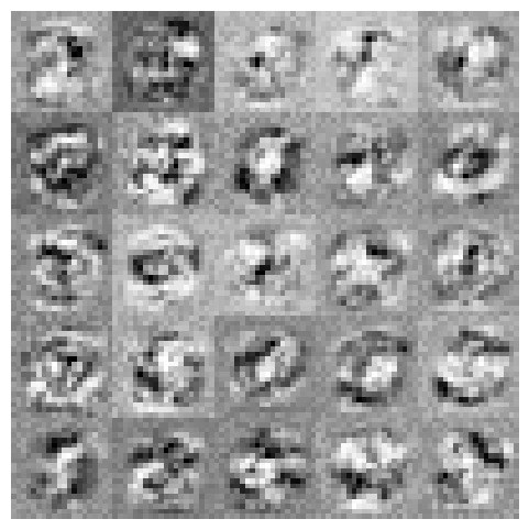
Image 4: Final output from hidden layer 5x5 grid
Key Steps:
The image above represents the hidden layer activations of our neural network. Each small square shows a pattern that the network has learned from the input data. These patterns, or feature detectors, help the model recognize handwritten digits by identifying key shapes, edges, textures, strokes, and digit-like structures.
By visualizing these activations, we gain insights into how the model processes data at different layers, improving interpretability and debugging potential issues.
In this project, we explored the fundamentals of neural networks, starting with forward
and backward propagation, optimizing weights using gradient descent,
and evaluating model performance on a labeled dataset. Through systematic experimentation,
we fine-tuned hyperparameters and observed how different activation functions and
architectures impacted classification accuracy.
A key takeaway from this project was the ability of the network to automatically learn
and extract features from raw input data. The final visualization of the hidden
layer activations provides insight into how the network perceives patterns within
the data. These learned representations, visible in the activation map, demonstrate the
network's ability to recognize edges, textures, and abstract features—which
ultimately contribute to accurate classification.
Moving forward, further improvements can be made by incorporating data augmentation,
convolutional layers (CNNs), or advanced optimization techniques to enhance feature
extraction and overall model performance.
I sincerely thank Prof. Andrew NG (DeepLearning.AI, Stanford University) for his inspiring courses that laid the foundation for this project.
 www.HoqueAi.com